Home - Techniek - Electronica - Radiotechniek - Radio amateur bladen - QEX - Accurate Measurement of Small Inductances
Build a bomebrew test oscillator for measufing inductance. Calculate L from the fixture's operating frequency.
When I embarked on a major project to build an amateur-band receiver, a number of interesting and a few difficult problems arose. Almost all of those issues could be addressed a priori because of the richness of the literature, but there was a notable exception. I lacked access to laboratory-standard test equipment-which is the case with most hams I expect. How does one measure small inductances with a precision of at least two, and possibly three, significant digits?
A search of the literature produced scanty results. One interesting circuit was described in The 2001 ARRL Handbook on p 26.22. I built a replica, and duplicated the results. Measurements with accuracy of ±10% can be made with that clever device from about 3 to 3000 µH, and that is good enough for many ham applications. A more accurate and direct reading device was described by Robert Vreeland, W6YBT, in QEX (May 1989); but an expensive Fluke DMM is required. Evidently, accuracy in the 3-5% range can be expected with W6YBT's elegant method. Nonetheless, 1% accuracy and measurement of smaller inductors (down to about 0.5 µH) was the goal, even if elusive.
I attempted numerous approaches, including various unsatisfactory bridges and the old standby grid-dipper method. By forming a parallel resonant circuit with a known-value capacitor and finding the resonant frequency with a grid-dip meter, the value of the inductor can be estimated. At best, this yields ±10% accuracy. A serious shortcoming of this method is that coupling to toroidal inductors is nearly impossible since the magnetic field is concentrated in the core. (Did I miss something? Has someone found a way to do this without influencing the unknown tuned circuit's resonant frequency?) Finally, a simple solution occurred to me: the converse of the grid-dipper method. If we put the unknown inductor in parallel with a known capacitance in an oscillator and measure the frequency of oscillation with a counter or accurately calibrated receiver, we can calculate the inductance from the known tuned circuit capacitance and oscillator frequency. This method works very well, and I am convinced that it yields measurements of very good accuracy using equipment and common parts available to the average ham.
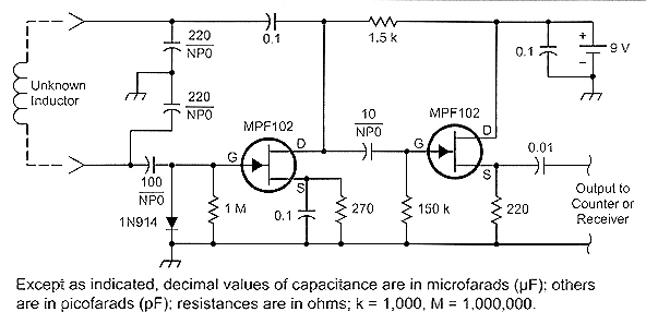
Fig 1: L-meter schematic diagram. Resistors are ±5% metal film; 5% NPO capacitors are used in frequency determining locations.
A simple - and admittedly ugly - breadboard was built on a small scrap of PC board. Fig 1 shows the circuit diagram, and Figs 2 and 3 are photographs of the breadboard and some of the inductors used to test it.
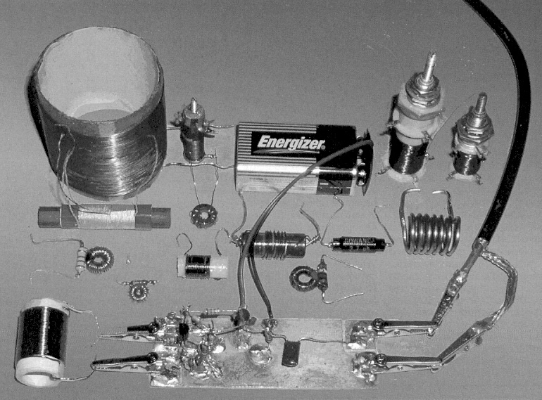
Fig 2: The "ugly" breadboard and typical inductors. The unknown inductor is connected to the alligator clips on the left. The counter or receiver is connected to the clips on the right via a shielded cable.
The circuit is a Colpitts oscillator followed by an isolating source follower. The junction FETs are MPF-102s, and all frequency-influencing capacitors are zero temperature coefficient (NPO) ceramics. Metal-film resistors are used for their stable RF characteristics, but exact values are not critical, so ±5% resistors will do nicely. Megohm resistors with one end soldered to the PC board are used as standoff insulators where needed. A 9-V battery provides power. Small alligator clips are soldered directly to the board for connection to the unknown inductor and for connection to the frequency counter or receiver. Half-inch square pads were etched into the copper with a small drill for the ungrounded alligator clip connections. Among other considerations, pay careful attention to minimizing series inductance in the tuned-circuit path. The small clips appear to be suitable for the inductance range of interest. The circuit in Fig 1 is satisfactory over the range of 0.5 µH or less to over 1 mH. The oscillator operates reliably over the range from a few hundred kilohertz to over 25 MHz. The signal level does fall off at the high-frequency (low-inductance) end, but there is sufficient output to drive a counter or to be heard in a receiver. Some unknown toroidal inductors from the junk box were reluctant to support oscillation-possibly because of low Q, but well-characterized ferrite and iron-core toroids worked in the circuit, along with a variety of other types as shown in Fig 2. Fig 3 is a closeup view of the breadboard-not pretty but competent.
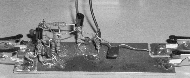
Fig 3: A close-up view of the "ugly" breadboard. The PC board's copper foil is circuit ground. Megohm resistors with one lead soldered to the foil serve as standoff insulators. The ungrounded alligator clips are soldered to hand-etched pads. Component leads in the oscillator circuit are kept as short as possible.
I intended the circuit for direct connection to a frequency counter, but very loose coupling to a general-coverage receiver can be used if a counter is not available. Disconnect the receiver from its antenna to minimize reception of interfering signals, then connect the output to the receiver through coaxial cable and a gimmick coupling capacitor consisting of a few twisted turns of insulated hookup wire. A receiver with digital frequency display is as good as a counter in this application. Keep in mind that the displayed frequency in some receivers may be offset from the receiver's oscillators, and you must zero-beat them with the test oscillator signal. You must make this correction if so. Receivers with analog dials will need calibration accuracy of four significant figures to achieve the desired measurement accuracy. (Many analog receivers meet that requirement.) It is possible, of course, to detect harmonics of the oscillator frequency, so a rough idea of the unknown inductance will put you near the right frequency.
To distinguish the fundamental from its harmonics, the lowest (and strongest) frequency you can detect is most likely the fundamental, and you should detect its harmonics only at exact multiples of the fundamental frequency. To obtain the desired accuracy, it is necessary to determine the actual value of the capacitance across which you will connect the unknown inductor. In the circuit shown, that value should be on the order of 110 pF. Here's how to determine the actual value of the input capacitance including all stray reactances. You will need a test inductor, preferably about 10 µH. The exact value is unimportant because it will cancel out in the following calculations. You will also need a calibration capacitor of known value in the range of 100-150 pF. You can probably trust a 1% NPO capacitor; but since many inexpensive digital multimeters claim to measure capacitance to 1% accuracy, make a measurement if you can to be sure. Better still, if you have a number of like 1% candidates of the same indicated value, select the one nearest the average measured value; then the accuracy of the multimeter doesn't matter. Statistically, the capacitor nearest the average value will probably be closest to the indicated value even if the DMM is off a bit or two.
Insert the test inductor in the alligator clips and measure the oscillator frequency with a counter or receiver. Then put the known calibration capacitor in parallel with the inductor. This can be done by inserting it in the clips along with the inductor, but it is better to tack-solder it directly on the board temporarily. Then measure the new, lower frequency. Since the frequency of a tuned circuit is inversely proportional to the square root of the capacitance, we can calculate the input capacitance as shown in Eqs 1 and 2:
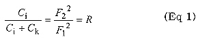
Where Ci = unknown input capacitance of the oscillator.
Ck = known capacitance
F1 = frequency with Ci only
F2 = frequency with Ck added to Ci
R = the ratio of the frequencies squared
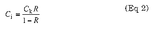
From the ratio R, and the value of the known capacitor, we compute in Eq 2 the input capacitance:
Now, with a known Ci we can compute the value of an unknown parallel inductance from Eq 3, the resonance formula:
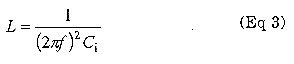
where f is the measured oscillator frequency and L the unknown inductance.
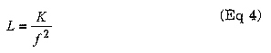
To simplify future calculations, we can establish a constant calibration factor for the device to compute L more directly:
where
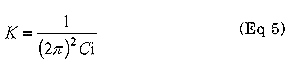
The dimension of K in Eq 5 can be adjusted to yield inductance in microhenries from frequency in megahertz.
Here's an example based on my breadboard. I used an inductor estimated to be about 10 µH from previous measurement attempts and a selected 100-pF calibration capacitor. As noted above, the actual value of the calibration inductor is unimportant because it cancels out in the calculations. The frequency of oscillation with the inductor only was 4.565 MHz. When the 100-pF capacitor was added in parallel, the measured frequency was 3.325 MHz. R, the ratio of the frequencies squared, was computed as 0.5305 according to Eq 1. Then using R = 0.5305 and Ck = 100 pF, the input capacitance was computed according to Eq 2 and found to be 113.0 pF. The calibration factor, K, was then computed according to Eq 5 and is 224.2. This gives Eq 6 for this specific device:
where L is in microhenries and f is in megahertz.
Using the same inductor to demonstrate the measurement process, we see from above that the measured frequency with the inductor alone was 4.565 MHz. From Eq 6, we compute L as 10.76 µH, and we round it to 10.8 µH. Don't trust that fourth digit since the calibration capacitor's value is known to only three significant digits. Notice, however, that by using four digits in all calculations, we minimize cumulative rounding errors in the third digit of the result.
To provide confidence in the calibration method, Ci was measured using various inductors over the range of 0.5 to 50 µH-two orders of magnitude. It does vary slightly due to differences in stray capacitance in the inductors, in this case between a computed minimum of 112.7 pF and maximum of 114.7 pF. That's about 1.5% difference. The average value of measured C. over this range was 113.7 pF, and the average value of K was 222.9 µH/MHZ2 . The measurement data and computations are shown in Table 1. All of the measured Ks up to 50 µH fall within 1% of the average value. So, we can use the average K of 222.9 in this range, retain some confidence in that illusive third digit of precision and swear to the second digit under oath.
Apparently, the device provides repeatable measurement accuracy approaching ±1% in the range of 0.5 µH to 50 µH using the common K factor. If inductors above this range are measured, the accuracy declines, but the common K factor is still useful up to 1000 µH or so, if high accuracy is not required. The difficulty in measuring inductance of larger inductors is caused by their significant interwinding capacitance. If accurate measurement of a given inductor is required, a unique K value can be determined for that inductor, thus treating its self-capacitance as a contributor to the input capacitance, Q. Three examples of this are shown ati the bottom of Table 1, and it is obvious that their contribution to input capacitance is significant. In fact, a good estimate of the self-capacitance of such an inductor is the difference between its uniquely computed C, and the average value of C. obtained with the smaller inductors that have little self capacitance. For example, the second listed of the three larger inductors in Table 1 shows a Ci of 121 pF compared to an average of 114 pF for the smaller inductance group, indicating that this inductor has about 7 pF of selfcapacitance. [Remember that the 7 pF travels with the inductor to its application circuit. Therefore, it is probably more useful to measure its inductance the first way, without consideration of the self-capacitance.-Ed.] The circuit could be optimized for these larger inductors since it is simple enough to construct large, intermediate, and small inductor versions. Some day I'll build three "pretty" versions with optimized configurations for each inductance range. Taken to the extreme, an automated device with direct reading digital display could be constructed. Below 0.5 µH, the error may increase due to series inductance but the device is still useful. That is another problem for another day.
Now, I will endeavor to finish the project that led to this diversion. In the meantime, please let me know your results if you experiment further with this method.
The measurements and calculations validate the use of a common K factor in the range of 0.5 to 50 µH. The dK and dK% columns represent deviation from the average value of K The values for the larger inductors at the bottom of the table were computed using their independent K factors.
| f1 (Mhz) | f2 (MHz) | R | Ck (pF) | Ci (pF) | K (µH/MHz2) | dK | dK% | L (µH) |
|---|---|---|---|---|---|---|---|---|
| 23.03 | 16.83 | 0.5340 | 100 | 114.6 | 221.0 | 1.87 | 0.84 | 0.420 |
| 21.63 | 15.81 | 0.5343 | 100 | 114.7 | 220.8 | 2.05 | 0.92 | 0.476 |
| 16.35 | 11.93 | 0.5324 | 100 | 113.9 | 222.5 | 0.41 | 0.18 | 0.834 |
| 15.34 | 11.18 | 0.5312 | 100 | 113.3 | 223.6 | -0.70 | -0.32 | 0.947 |
| 8.999 | 6.556 | 0.5307 | 100 | 113.1 | 224.0 | -1.08 | -0.49 | 2.75 |
| 4.565 | 3.325 | 0.5305 | 100 | 113.0 | 224.2 | -1.29 | -0.58 | 10.7 |
| 4.508 | 3.285 | 0.5310 | 100 | 113.2 | 223.7 | -0.85 | -0.38 | 11.0 |
| 3.443 | 2.506 | 0.5298 | 100 | 112.7 | 224.8 | -1.96 | -0.88 | 18.8 |
| 3.057 | 2.227 | 0.5307 | 100 | 113.1 | 224.0 | -1.12 | -0.50 | 23.8 |
| 2.293 | 1.674 | 0.5330 | 100 | 114.1 | 222.0 | 0.91 | 0.41 | 42.4 |
| 2.009 | 1.468 | 0.5339 | 100 | 114.6 | 221.1 | 1.77 | 0.79 | 55.2 |
| Average | 0.5320 | 113.7 | 222.9 | |||||
| 1.482 | 1.089 | 0.5400 | 100 | 117.4 | 215.8 | 98.3 | ||
| 0.8185 | 0.6054 | 0.5471 | 100 | 120.8 | 209.7 | 313 | ||
| 0.5035 | 0.373 | 0.5488 | 100 | 121.6 | 208.3 | 821 | ||
AK4AA.