Home - Techniek - Electronica - Radiotechniek - Radio amateur bladen - QST - Modulation in Radio Telephony
Here at last is really authoritative information for the amateur on radiophones. Mr. Heisiag has given the amateurs a splendid paper couched in terms they can understand and we consider it the best article on the subject it has yet been our pleasure to present. Incidentally it should settle once and for all the argument about grid leak vs. constant current modulation.
The Modulated Antenna Current
The average radio amateur on entering the radio telephone field, must bear in mind the fact that he has much to learn to make a satisfactory telephone set that was not necessary for a telegraph set. Also, that because the nature of the signals to be transmitted is different, certain methods of operation and certain requirements which were proper for telegraphy are decidedly improper for telephony. Neglect of these facts and a blind effort to apply to telephony the rules for telegraphy will result in a considerably poorer set than should be the case.
Before discussing any of the systems of modulation, it appears desirable to point' out some of the essential facts concerning radio telephony. By doing so, the reason for many modulation circuit connections will be better understood and the finer points which distinguish a poor arrangement from a good one will be appreciated. A study of the form of the antenna current as influenced by a signal will give us many pointers as to the best arrangements for a good circuit.
Human speech, which is the signal to be transmitted in radio telephony, consists of an aggregation of frequencies lying largely between 200 and 2000 cycles per second, having various amplitudes, periods of duration, and transients at the beginning and end, so arranged as to convey information to the listener. To convey the human voice by radio it is necessary to provide a system which will convey all of these frequencies; that is, it must reproduce each frequency at the receiving end and reproduce it with the proper amplitude in comparison with the others, and reproduce its "transient" or amplitude variation at the beginning and the end, and it must do this for each frequency while doing it for others. This is enormously more difficult than transmitting a telegraph signal. To transmit a telegraph signal it is only necessary to produce some kind of a noise at the receiving station and the signalling is done by varying the duration of this noise. The noise does not have to bear any relation to any noises at the transmitting station but needs only to be something the receiving operator can hear. In telephony, any noise will not do, because the noise to be reproduced must be identical with the noise produced at the transmitting station, it must contain the same frequencies, give them their relative amplitudes, and have them last the proper length of time. The complexity of the signal necessitates a control of the radiated wave not necessary in a telegraph system and it is the control which is such an important part of the radio telephone circuit.
An example of a radio telephone wave is indicated in Figure 1. The carrier wave amplitude is here varied according to the wave form of the signal. The precision of control required to cause the proper antenna current, regardless of the millions of forms the signal may take, is quite evident. This signal on being received and rectified will reproduce the modulating signal, since the rectified current will be substantially proportional to the high frequency amplitude.
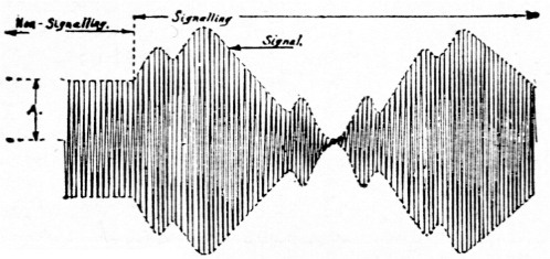
Fig. 1. H.F wave modulated by speech signal.
In the discussion of a radio frequency current, it is usual to assume a simple signal as the modulating signal, as most of the necessary information can be secured with that assumption. It is assumed that the signal to be transmitted is a single sine wave of some audio frequency such as 800 cycles. A modulated antenna current carrying this signal is represented in Figure 2. This antenna current is expressed by the equation
![]()
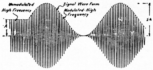
Fig. 2. HF-wave modulated by a single sine wave signal.
In this equation sin wt represents the radio frequency wave and sin pt the signal frequency wave. K is known as the modulation constant and is usually expressed in percentage form. When no signal is being transmitted the high frequency amplitude is A and the constant K is zero. If a signal of such a loudness as to make K equal to unity is spoken, the term 1 + k sin p t varies between values of 0 and 2 depending upon sin p t passing through the values -1 and +1- and the amplitude of the high frequency current varies between zero and 2A. That is, the modulation of the current causes it to rise, as well as fall, and it should rise as much above as it falls below. If the system is so constructed that the amplitude does not rise, but is varied downward only, a speech signal will produce a wave of the form shown in Figure 3. Inspection of this indicates that a great distortion is produced. The amplitude should vary so as to follow the dotted signal line, but the failure of the system to cause the current amplitude to rise chops off one-half of the speech signal and gives an imperfect reproduction at the receiving end. This one-sided or improper modulation is to be avoided if possible.
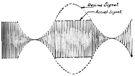
Fig. 3. An improperly modulated wave.
Those who are acquainted with elements of trigonometry will observe that we can change the form of the equation (1). Such a change does not affect its validity at all but does point out one or two new facts. The equation can be changed to:

This equation indicates that a sustained wave, such as shown in Figure 2 and represented by equations (1) and (2), can be said to consist of three frequencies:
The radio carrier frequency ![]() of amplitude A.
of amplitude A.
An upper side frequency ![]() of amplitude
of amplitude ![]() .
.
When no signal is being transmitted, K = 0 and the only frequency is the radio carrier frequency with amplitude A. As soon as the signal begins to modulate the wave, the side frequencies ![]() and
and ![]() of amplitude
of amplitude ![]() appear while the carrier remains unchanged. The modulation of the radio wave thus takes the form of the production of side frequencies. At the receiving station, the beats between the carrier frequency and the side frequencies, when rectified, produce the frequency of the transmitted signal.
appear while the carrier remains unchanged. The modulation of the radio wave thus takes the form of the production of side frequencies. At the receiving station, the beats between the carrier frequency and the side frequencies, when rectified, produce the frequency of the transmitted signal.
If the signal to be transmitted consists of many frequencies such as 200, 500, 1200, and 2000 cycles, the frequencies in the antenna will be the carrier frequency f and the side frequencies f + 200, f - 200, f + 500, f - 500, f + 1200, etc. In telephony, human speech contains frequencies largely between 200 and 2000 cycles so that to transmit speech by radio we must expect to have in the antenna the carrier f and the side frequencies f + (200 to 2000) and f - (200 to 2000). That is, if we use a carrier of 50,000 cycles there will occur in the antenna the frequencies:
The carrier 50,000 cycles
Lower side frequencies between 48,000 and 49,800
Upper side frequencies between 50,200 and 52,000
giving us a band 4,000 cycles wide necessary for the transmission of speech.
Having described in detail the important features of a radio telephone wave, we are now in a position to point out a few facts of vital interest to an amateur. In radio telegraphy, it is customary to tune and adjust the set for the maximum antenna current that it is possible to obtain. Signalling is then done by making and breaking the circuit causing the antenna current to fall to zero in the spaces and rise to the maximum in the dots and dashes. The greater the antenna current, the greater is the VARIATION in the current when signalling. The VARIATION in the current is what is desired and the maximum antenna current is tuned for only because the change in current between that value and zero gives the greatest VARIATION. The VARIATION in the current while signalling is thus the factor which determines the loudness of the received signal. In telephony the VARIATION in the antenna current while signalling is also the determining factor as regards loudness of signal or distance to be reached, but the amateur must remember that the determination of the maximum VARIATION is not so easily done as in the case of telegraphy. The antenna current is not merely reduced to zero in spaces and then returned to the normal value, but it varies through all possible values from zero to TWICE THE NON-SIGNALLING VALUE. In telegraphy the current is either zero or maximum. In telephony it has a certain non-signalling value (A in equation 1 and Figure 2) and takes all possible values between 0 and twice the non-signalling value (2A in equation 1) and the apparatus must be capable of producing any possible value between these limits. Therefore the amateur is warned that when he tunes his set up for the non-signalling value A, he must see that the system that he uses has some variable in it which when operated upon by the speech will make the set give 2A in the antenna. Failure to remember this will result in producing one-sided modulation as shown in Figure 3.
In telegraphy, it is possible to determine with the antenna ammeter alone the VARIATION in antenna current while signalling. When the key is open the current is zero, when it is closed the current is a maximum. In telephony, unfortunately for the amateur, there is no simple apparatus to tell what the variation is, or to tell him when he is getting complete modulation. There are, however, two indicators which will give an operator some idea of his degree of modulation. The first is the variation in the reading of the antenna ammeter. When a wave is completely modulated by a symmetrical signal in a properly adjusted set, the antenna ammeter reading increases by about 22½ %. (To be exact, the reading is V (1.5) times the non-signalling value). This must not be taken as an infallible guide as it is not easy to get a set adjusted so as to make this indicator worth much. A badly distorted wave will give a reading variation of even greater than this amount. Judgment should not be passed upon this evidence alone. The second indicator is the quality of the received signal. The signal from a set which tends to "over-modulate" has a peculiar sound often described as "tinny". It sounds like the voice of a person holding a sheet of paper against the lips. It is caused by the over-modulating action cutting off the peaks of certain loud signal waves. The identification of this kind of distortion can be learned by observation. The amateur must not let his imagination get the better of him and confuse microphone distortion or other noises and distortions with this over-modulation distortion as many do. He should learn to identify the sound under conditions that will not give him the wrong impression of its character. This indicator is the only cheap indicator of complete modulation at present available to the amateur. It is much more reliable than the antenna ammeter method, but indicates only over-modulation. It will be found, however, to be useful.
Having discussed the nature of a modulated antenna current, we are now in position to discuss some of the systems which produce it.
Colpitts system
Among the systems of modulation which may be of interest may be mentioned Colpitts' system shown in Figure 4 and a modification of it, the Logwood system shown in Figure 5. This system is primarily an oscillator upon the grid of which the speech signal is impressed. In this circuit the grid acts as control member for the amplitude of the oscillation. However, as the grid is also used for controlling the current through the tube while oscillating, it is compelled to perform two different functions simultaneously and unless the circuit is very carefully adjusted, it fails in either one or the other. Usually the amateur will adjust the oscillator to get the most power into the antenna and then impress the signal upon the grid expecting perfect operation as easily as is secured in telegraphy by opening and closing the key. Such, however, is not what results. This system gives about 20% modulation, which is quite poor. To adjust this circuit to give complete modulation requires much more complicated apparatus that the amateur is likely to possess, and there is added the fact that the adjustment is not only difficult to obtain, but is difficult to maintain. The efficiency of such an arrangement is not very high. For an amateur who wishes to secure good range the system is not advised. If, however, one is merely interested in something which will talk a short distance, it is one of the easiest systems to construct.
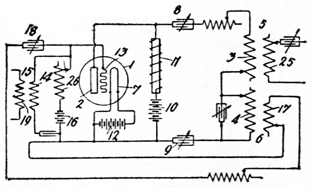
Fig. 4. Colpitts system.
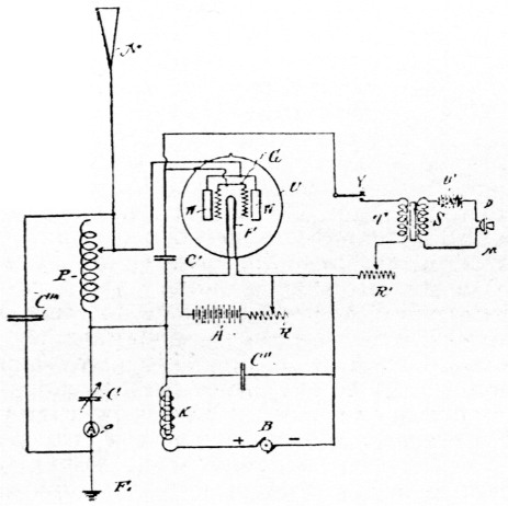
Fig. 5. Logwoods circuit.
Van der Bijl system
A system which we have used in many of our experiments is shown in Figure 6 and is known as the Van der Bijl system. It falls under a classification of systems known as "amplifier systems" in which a small amount of power is modulated and then the modulated current is amplified into the antenna. The modulation is done in this circuit by means of a tube in which we make use of its curved characteristic. In Figure 6 will be observed a small high frequency voltage with the time axis running downward, which is impressed upon the grid and whose position on the characteristic curve is varied by the signal to be transmitted. The varying slope of the characteristic curve causes the high frequency current in the plate circuit to change, depending upon what part of the characteristic curve this small voltage wave operates. If it operates around the point marked B, it produces the amplitude indicated directly to the right of the letter B. If it operates around the point marked C, it produces a much greater amplitude as is indicated to the right of that letter. If the signal should slide this wave down to the point A, practically no alternating space current occurs. We thus have the phenomenon of being able to get any alternating space current we desire by merely sliding the high frequency input up and down the curve. If we use the signal to slide this small input up and down, the amplitude produced in the plate circuit is such that a line drawn through the peaks (the envelope of the peaks, so to speak) is the wave form of the signal desired. Having once secured a small amount of modulated high frequency current, it is only necessary to amplify it up to the desired power and put it on the -antenna.
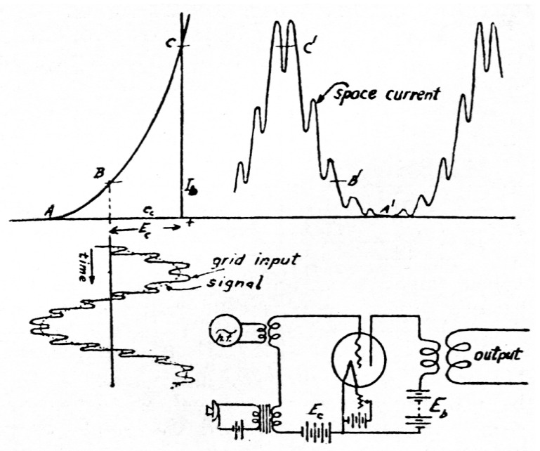
Fig. 6. Van der Bijl's system.
This type of system, though fairly simple, is not as good as some to be described later. It is however, as good and as efficient as any other amplifier system. That is, it is as good as any system in which a small amount of power is modulated by some means and then amplified to the desired point. The efficiency in these systems is determined by the efficiency of the amplifier and has very little connection with modulating arrangement itself.
The circuit which we used in our test at Arlington, 1915, is given in Figure 7. The average amateur should be able to pick out the oscillator, modulator and amplifiers in this circuit without much trouble.
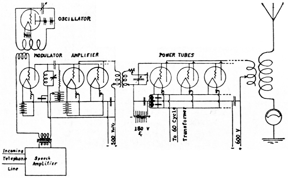
Fig. 7. Arlington experimental circuit
Modulating Amplifier System
A modified form of the Van der Bijl system is that indicated in Figure 8. It is known as the "modulating amplifier" system. It differs in detail from the previous arrangement in that the high frequency wave impressed upon the grid is equal to or much larger than the signal wave, instead of being much smaller, and in that the modulator not only modulates, but amplifies and delivers the modulated high frequency current directly to the antenna. This system should be of some interest to an amateur because it is one he can quite easily construct. It requires, however, two or more tubes. One of the tubes must be used to generate the high frequency oscillations, while the other is used as the modulating amplifier. These tubes may be of different sizes; the one generating the high frequency oscillations does not have to be over 1/10 the power rating of the modulating amplifier tube. If the tubes are of very large size, it may be necessary to use a speech amplifier between the microphone and the modulating amplifier.
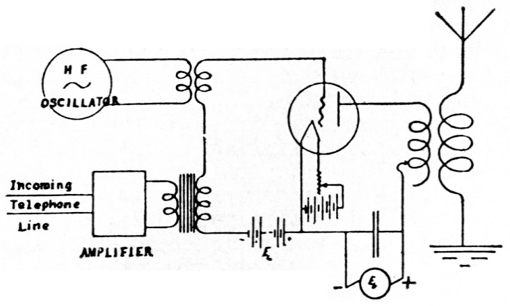
Fig. 8. Modulatitt amplifier circuity.
In a system of this kind, it is desirable to have a high frequency amplitude several times the signal frequency amplitude. The experimenter should vary the negative voltage , finding the values at-which he gets maximum current and minimum current in the antenna. After having determined these values, he should set the negative voltage at about the value halfway between these limits, the value being that which will give 1/2 the maximum antenna current. The circuit it then properly adjusted for speech since the non-signalling value is ½ the maximum possible. He must not feel that he is cheating himself out of some power when he reduces the antenna current to half the maximum, because he is not. The speech signal coming in. and being impressed will momentarily oppose the battery at times and cause the power to rise to the maximum, and at other times will momentarily aid the battery, causing the power to decrease to zero. He has a value about which the antenna current can both increase and decrease by the mere changing of the potential of the grid. This gives him a circuit adjustment which will produce an antenna current as indicated in Figure 1 or Figure 2. It can rise to a higher value as well as decrease to a lower value by a mere potential change which in this case is his grid potential, and he can get a properly modulated, if not a completely modulated, antenna current. The natural inclination of the amateur is to leave the value of Er such as to give him the maximum antenna current. If he does this, he can only secure an improperly modulated current such as in Figure 3. His signal impressed from the transmitter and the transformer has alternating potentials which in some instances aid the battery Ec, and other instances oppose it. At those instances where it aids the grid battery and makes the grid become more negative, the antenna current will be modulated in a downward direction. But in those instances when it opposes the grid battery and reduces the grid potential it should raise the antenna current. If he does not make the non-signalling antenna current half the maximum by increasing the negative grid battery he will be operating about the point of maximum antenna current and nothing he can do on the grid can ever make the current any greater. Since his speech signal contains equal amounts of positive and negative potentials which alternately aid and oppose the battery, he will get modulation only for that half of the signal which aids the battery, giving him the identical improperly modulated signal represented in Figure 3. To secure the complete radio signal, he must increase his negative grid voltage to such a value. as mentioned previously, as will allow the incoming speech signal to oppose the battery and increase the antenna current at times as well as to aid it and decrease it at other times.
A set of curves such as a person would get from a modulating amplifier is indicated in Figure 9. The curve for antenna current (I.) was secured by slowly varying the negative grid potential and taking readings of the antenna current at the same time. As we approach the value of 100 volts on the grid, it is seen that the antenna current is rising so slowly that it is not desirable to go any farther in that direction. In fact, for most work, it is better not to go to a smaller value than 200 volts. This is marked by the letter Z. Half way between this value and that value W at which the antenna current is reduced to zero is marked the value X which is the amount of negative voltage we would apply to the grid when not signalling. If now. we produce by means of a microphone and transformer the simple signal indicated with the time axis running downward, we can cause the potential of the grid to vary. The potential of the grid is the sum of the constant negative potential 280 volts and the varying signal potential, and the grid's potential will range between the points W and Z, causing the high frequency antenna circuit to vary between the maximum and minimum values.
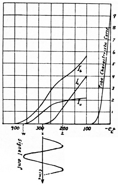
Fig. 9. Behavior curves for the modulating amplifier.
Constant Current System
The most desirable circuit for most amateurs to use is the constant current system. This has been described in numerous papers .but is indicated again in Figure 10. It consists essentially of an oscillator and a modulator tube being supplied in parallel from a constant current source. The constant current source needs to be of constant current only as regards the signalling frequency, and then, does not have to be exactly so, but merely relative. The simplest arrangement is indicated as consisting of a constant potential generator with a large choke coil in series. Any variation of current through the generator and choke coil at the signal frequency is enormously opposed by the large choke coil, so that if a signal is impressed upon the grid of the modulator tube causing the current taken by it to vary, the variation must pass through the oscillator for the reason that the large choke coil imposes such a large impedance to any variation in current through the generator that the variable current is forced through the oscillator.
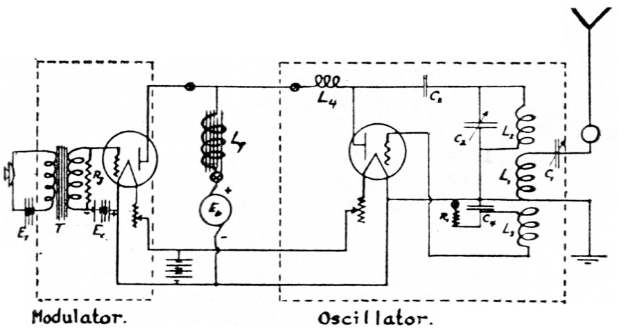
Fig. 10. 200 Meter constant current transmitter.
This causes the oscillator to deliver an antenna current which varies according to the power supply.
The behavior of the constant current system is represented in Figure 11. The modulator has such a negative voltage that its space current is about the same as that of the oscillator. Theoretically they should be exactly the same but practically the modulator can be adjusted to take one half the space current of the oscillator when not signalling and on account of the curvature of the tube's characteristic, it will rise to an equal value while signalling. In curve I they are represented as equal. The top horizontal line represents the total space current which is kept constant. As the signal is impressed upon the modulator grid, the current taken by it varies according to the distance between the curved line and the top horizontal line, forcing the oscillator to take the remainder of the current-that represented by the ordinates of the curved line-from the bottom horizontal line. Now the voltage necessary to force this varying current through the oscillator must vary also, and it happens to vary in a corresponding manner, having the form shown in curve II. The antenna current amplitude is proportional to the oscillator voltage or to the oscillator current and will also vary in a corresponding manner as shown in curve III. We thus get in the antenna a h.f. current whose amplitude varies according to the signal to be transmitted.
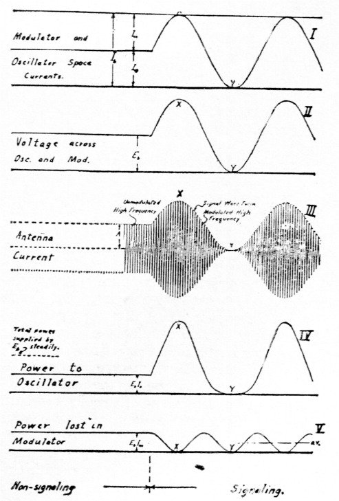
Fig. 11. Constant current system Behavior curves.
The reason for the rise in voltage at point X to twice the generator voltage is explained by the fact that the constant current choke coil acts as a storehouse for energy at times and delivers this energy back at other times. Thus at point Y curve II the voltage across the oscillator and modulator is practically zero because the modulator resistance has dropped and the choke coil has such a large reactance against an increase in current that most of the generator voltage, if not all, is taken up by it. During this period, the choke coil stores up energy being delivered by the B battery. At other instants such as X, the modulator resistance has gone to infinity and the choke coil now delivers up this stored energy and causes the voltage across the oscillator to rise to twice the normal value.
The variation of power to the oscillator is represented in curve IV. This curve is arrived at by multiplying curve I by curve II. An interesting fact to be observed is that at point X the power being delivered to the oscillator is twice the average being delivered by the B battery. This is accounted for by the fact previously mentioned of the choke coil storing up energy during part of the signal cycle (around point Y) and delivering up this energy at another time. It causes the constant current system to be one of the most efficient circuits that has been devised.
Curve V represents the power delivered to the modulator. The power lost there is a maximum under the non-signalling condition. At point X when all the current goes to the oscillator and none to the modulator, the power dissipated in the modulator is zero. At point Y when all the current goes to the modulator and none to the oscillator, the voltage across the modulator is so small that again scarcely any power is lost there. Thus at the two extremes of maximum and minimum antenna current, the modulator dissipates no power, and the average while transmitting a completely modulated signal is one half the non-signalling amount wasted.
A desirable feature of this system is that no further changes or adjustments are necessary to the oscillator after tuning it up properly. The modulator is not part of the high frequency circuit and upon completing the high frequency adjustments, the system is ready to work.
It must be remembered, however, that the modulator has its own adjustment-that of the negative grid potential-bat this adjustment is independent of the high frequency circuit.
This system can be used with any type of oscillator, or with certain masteroscillator-controlled amplifiers. The principal precautions to be observed are to see that the high frequency and audio frequency circuits have proper condensers or choke coils in them to pass the desired currents and stop the undesired ones.
R. A. Heising.