Home - Techniek - Electronica - Radiotechniek - Radio amateur bladen - QST - A simple and accurate QRP directional wattmeter
Make a few small enhancements to the Bruene wattmeter and diode detector, and you have a directional wattmeter that's simple, portable, and accurate from 10 watts down to 5 milliwatts!
A directional wattmeter is a really indispensable tool. Besides using such a meter to measure SWR, you can use one to tune a home-built rig, adjust a Trans-match, measure cable loss, and a host of other things. Because it's portable, a wattmeter is an important tool in the field: With it, you can make sure the rig still works, and spot any problems with the antenna system. If you're operating QRP in Field Day or some other event, a good wattmeter can help you keep your output at five watts as the battery voltage drops.
This wattmeter, designed primarily for portable use, gives accurate readings at power levels from 5 mW to 10 W. Achieving good low-power accuracy is a bit tricky; I developed a simple correction circuit to handle the job. During the editing of this article, I learned that the technique I developed for compensating the diodes in this wattmeter's detector circuit was first discussed by John Grebenkemper, KI6WX, in his January 1987 QST article.(1) I encourage reading (or rereading) this excellent article.
If carefully constructed, this wattmeter should function well from below 1 MHz at least into the mid-VHF range. One prototype tested in the ARRL Lab maintains better than ± 70/e of full-scale accuracy, on all ranges, up to 432 MHz.
Circuit description
A basic directional wattmeter has three major parts: directional coupler, detector, and meter circuits. Each block can be optimized for a particular application. Here's a description of each block.
Directional coupler
Two types of directional couplers are commonly used by amateurs. The venerable Monimatch circuit is simple and useful for SWR measurement, but not readily adaptable as a wattmeter except over a narrow frequency range, because its sensitivity changes with frequency.(2) The Bruene circuit doesn't have this limitation, so is more suitable for our use. It's generally implemented with capacitive dividers for sensing voltage, but I chose to use transformers for this function.(3) This results in a simpler circuit that's adjustment-free. Sensitivity can be traded for insertion loss; the values chosen for this meter result in insignificant insertion loss.
Maintaining a near-50-Ω impedance on the line through the wattmeter eliminates several frequency-dependent effects. A microstripline structure is effective for this application, and is extremely simple to build, so I used that technique in this wattmeter.
Ac v. Dc: Why the Difference?
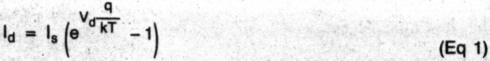
Why does a diode detector produce less output when detecting an ac signal than a dc signal if both signals have the same peak value? Why does a pulsed-dc signal produce a lower output than a steady one? Fortunately, we don't have to look any further than the ideal-diode equation to get the answers to these questions. This equation describes the characteristics of an ideal diode - a diode that is ideal in the sense that it can be described by some fundamental principles, not in that its conduction is perfect in one direction and zero in the other.
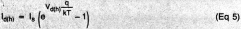
The ideal-diode equation is:
where
Id = Diode forward current
Is = Saturation current, about 10-14 A for silicon, 2 x 10⁻⁷ A for germanium at room temperature
Vd = Diode forward voltage
q Electron charge, 1.60 x 10⁻¹⁹ coulomb
k = Boltzmann's constant, 1.38 x 10⁻²³ J/K
T = Temperature, K
At room temperature, kT ÷ q is about 25 mV. Note that Is is strongly related to temperature, doubling with approximately every 10-°C rise in temperature.
Because our discussion primarily concerns small signals, let's see how the ideal diode behaves with small voltages or currents applied. The small-signal IN characteristics of an ideal germanium diode are shown in Fig A. This is simply a graphical representation of Eq 1 over a limited range. (The graph is also valid for silicon diodes if the current scale is reduced by a factor of about 20 million.) Note that the IN curve doesn't bend at the origin; it's a straight line. This gives us our first clue about small-signal diode operation: a straight line on an IN graph represents a constant resistance, so at very small signal levels the diode looks like a resistor, and hardly rectifies at all. (By very small signal levels I mean somewhat less than kT ÷ q [25 mV).) The resistance of the germanium diode is about 125 kΩ in this range (an ideal silicon diode is about 2.5 TΩ (2.5 x 10¹² Ω). At higher forward voltages, the current rapidly rises; at greater reverse voltages, the current increases, then levels out at a value of -Is.
If we apply dc to the circuit of Fig 1, current will flow heavily at first, then taper off as CL charges. Eventually, the current will simply be Vo ÷ RL. Substituting (Vi - Va) for Vd in Eq 1 and rearranging produces an equation relating Vo and Vi: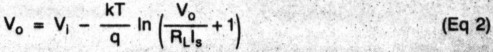
or Vd and Vo:
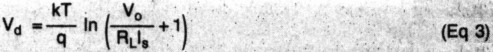
To get a feel for the voltage drop to expect, look at Eq 3 with Vo = 100 mV, RL = 1 MΩ, and Is = 2 x 10⁻⁷ A. This results in a diode drop (Vd) of 10.1 mV. In contrast, a silicon diode (Is = 10-14 A) would drop 403 mV (503 mV in for 100 mV out) under the same conditions, but it would have 10.1-mV drop if RL was made 20 million times larger. As the signal level increases, the drop increases - but not in proportion, so detector accuracy improves. Increasing the load resistance helps also; at 100 mV out and RL = 10 MΩ, Vd = 1.2 mV.
Now let's see what happens with an ac or pulsed-dc signal. Looking at Figs 2 and B, we can see that when Vi is greater than Vo, the drop is the same as if the input signal were dc. However, for part of the cycle, Vi is less than Vo. During this time the diode is reverse biased and substantial current flows to the left in Fig 1. Generally, CL is made large enough to make the ripple on Vo very small. We can then consider Vo to be a constant value after an initial charge period of many cycles of the input signal. For any signal,
![]()
where Id(avg) is the average current flowing through the diode over a cycle of the input signal.
The wattmeter's detector signal is a bipolar sine wave, but analysis of a unipolar square wave illustrates the principle and is much easier to attack mathematically (I'll discuss the sine-wave case shortly).
Consider a unipolar square wave with a positive value Vp for 50% of the cycle and 0 V for the other 50%. When the input signal is positive,
where
Id(h) = diode current when the input signal is high.
Vd(h) = Vp - Vo = forward voltage (diode drop) when the input signal is high.
This follows directly from Eq 1. When the input signal is zero, the diode is reverse biased. Again from Eq 1
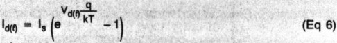
where
Id(l) = diode current when the input signal is low. Id(l) is negative.
Vd(l) = -Vo = diode forward voltage when the input signal is low. Vd(l) also is negative.
Because Id(h) and Id(l) each flow during 1/2 of the input cycle, average current is found by
![]()
Combining Eqs 5, 6, and 7 and solving for Vd(h):
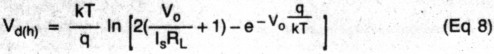
Vd(h) represents the difference between the peak value (Vp) of the input signal, and the output voltage (Vo). An analysis of the argument of the logarithm shows that it's always greater than the dc case. In fact, when Vo gets much greater than kT ÷ q, Vd(h) = Vd(dc) + (kT ÷ q) in (2), or about 18 mV at room temperature. This result is independent of RL, so even if RL is large to minimize dc drop, the added drop due to applying ac will stay the same (as long as Vo >> kT ÷ q). The added offset is clearly shown in Fig B. Values calculated from Eqs 1 and 8 fall almost exactly on the graphs. A similar analysis for a bipolar square wave results in the same limiting value of 18 mV of excess drop.
Math is fun! But everyone's got a limit, and mine falls within the large gap between analyzing the detector with square-wave and sine-wave inputs. However, some generalizations can be made without having to do a rigorous sine-wave analysis. With a sine wave applied, one would expect diode forward current to flow for only a small part of the input cycle, resulting in a greater drop than with a square wave applied. The sine-wave case was studied with a mathematical computer model, and the results agreed very closely with the measurements presented in Figs 2 and B. - W7EL
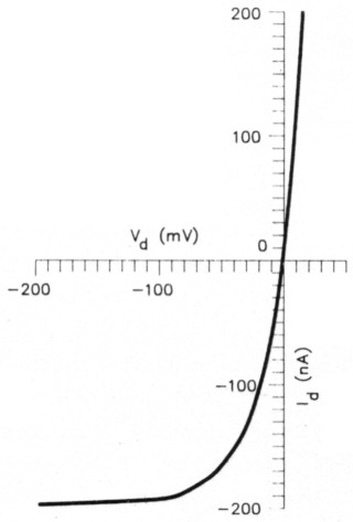
Fig A - Current-voltage characteristics of an ideal germanium diode.
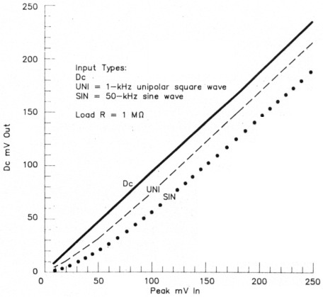
Fig B - The same data as that of Fig 2, plotted on linear axes.
Detector
Seemingly, the detector should be the easiest part of the wattmeter to design. Well, it happened again: The simplest part turned out to be the hardest. What's so hard about using a diode detector? If you don't want to know, skip ahead to the Construction section. For the truly adventurous (mathematically, that is), I've included the sidebar, "Ac v Dc: Why the Difference?"
Plain diode detectors, like the one shown in Fig 1, are simple and easy to use - provided you don't require accurate results at low signal levels. That's unfortunate, because good low-power accuracy is exactly what this wattmeter is intended to provide. Five milliwatts provides only 145 mV (peak) at the detector, so detector accuracy must be maintained down to this level. Some diodes, such as back diodes and zero-bias Schottky types, are specially designed for detecting very small signals. These, however, aren't as readily available as common silicon, germanium, and medium-barrier silicon Schottky diodes, so I investigated only the latter three types. Naturally, each has its deficiencies.
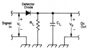
Fig 1 - Simple diode detector.
Common small-signal silicon diodes (eg, 1N914) drop too much forward voltage to be accurate at small signal levels when used with reasonable load-resistance values (up to 100 MΩ or so). Ordinary small-signal Schottky diodes are better, but still have an objectionable drop for use at low signal levels. The good old point-contact germanium diode (1N34 type) is the clear winner in this category. Applying 50 mV (dc) to a germanium diode detector produces about 45 mV at its output with a 1-MΩ load resistance. Increasing the load resistance to 10 MΩ brings the output to within 1 mV of the applied voltage.
So what's the problem? The problem is that the results are different when you apply an ac signal to the detector! This difference is clearly shown in Fig 2, which gives the measured output of a germanium-diode detector (like the one shown in Fig 1) with three different input signals of the same peak value. On the log-log scales, the vertical spacing between plots is proportional to the fractional (percentage) difference between the outputs. As you can see, a simple germanium detector is accurate for ac signals only when the peak input signal level is above about l V. A simple correction circuit is the secret to this wattmeter's accuracy. I'll explain it in a moment, but first I'll briefly explain why the detector output is less with an ac than with a dc input.
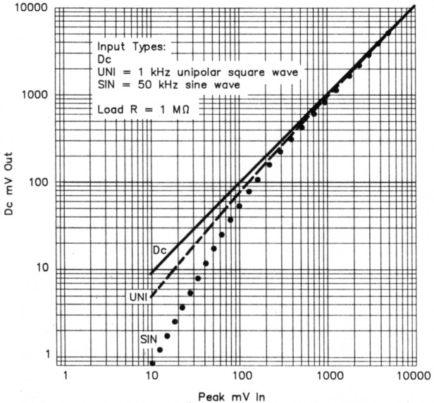
Fig 2 - Dc output voltage of the detector of Fig 1 with three types of input signals.
When the forward or reverse voltage across a diode gets very small (a few millivolts), the reverse and forward currents are approximately equal for a given applied voltage; that is, the diode acts like a resistor. (I measured a typical germanium diode's resistance as about 120 kΩ, a value very much smaller than that of silicon diodes.) If dc is applied to the detector, the detector circuit acts like a voltage divider, with the input voltage dividing be tween the diode resistance and the load resistance. When ac is applied, however, the current flow during the negative half-cycle removes a substantial part of the charge put on the load capacitor during the positive halfcycle, resulting in a lower detector-output voltage. The effect is waveshape and duty-cycle dependent, but isn't related to the frequency of the input signal.
Silicon diodes exhibit the same properties, but at different levels. Silicon-diode resistance at few-millivolt levels is about a million times larger than that of germanium diodes, but extremely large load resistances (1012 Ω or so) would have to be used to bring the forward drop to the germanium-diode level. The much smaller currents flowing through the much larger resistance result in the same net effect. The observed ac/dc difference is explained by the ideal-diode equation (see the sidebar). Dc and unipolar-square-wave measurements were compared to results predicted by the ideal-diode equation with extremely good agreement.
Common 1N34A germanium diodes purchased from Radio Shack were found to be satisfactory for this detector.
The Meter Circuit
See Fig 3. An op amp is a logical choice to provide a high load impedance for the detector and a low-impedance output. Most op amps, however, have enough input-bias current to produce a significant voltage across a high-value detector-load resistor, ruining the measurement. Fortunately, operational amplifiers that have input-bias currents of only a few picoamperes - more than adequate for this application - are readily available. The CA3160 (and its externally compensated equivalent, the CA3130) has the desirable combination of extremely low input current, input-and output-voltage range down to the negative supply rail and moderately low current consumption. To my knowledge, no other readily available op amp shares this set of features; if you know of one, you may substitute it for the CA3160 used at U1.
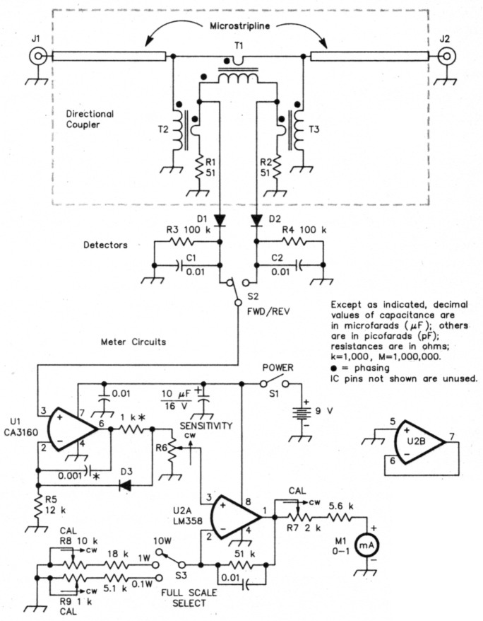
Fig 3 - Schematic diagram of the QRP directional wattmeter. All fixed resistors are 1/4-W, 5%-tolerance units. D1-D3 are common 1N34 germanium diodes; they should be matched (as discussed in the referent of Note 1) for best performance. T1-T3 are FT-37-72 ferrite cores with single-turn primaries (one pass through the core - see Fig 5). The primaries of T2 and T3 are comprised of the ungrounded leads of R1 and R2, respectively. Each transformer has a single secondary winding consisting of 10 evenly spaced turns of no. 28 enameled wire. Do not substitute a different core for the FT-37-72. R6 can be any value between 10 kΩ and 100 kΩ. The resistor and capacitor (associated with U1) marked with asterisks may be necessary to eliminate instability in the op amp, although my prototypes don't require them. See text.
The second op-amp input is used by the diode-compensation circuit, so a second stage is required to permit variable gain. The only requirements for the second op amp are moderate current consumption and the ability to handle input and output signals down to the negative supply rail (ground). The LM358 contains two such op amps; one section (U2B) is unused in this application. You could substitute one section of an LM324, another CA3160, or any other op amp having the required characteristics.
The diode-compensation circuit (D3 and R5 in Fig 3) creates an offset that approximately compensates for the drop across the detector diode. If dc was applied to detector D2/R4/C2, and if compensation resistor R5 and detector load resistor R4 were equal, perfect compensation would result (assuming that D2 and D3 were identical). However, the circuit is actually compensating the detector ac drop with a dc drop, so more current must flow through compensation diode D3. This is accomplished by making R5 smaller than R3 and R4. Although the compensation isn't perfect, it's extremely good, and a remarkable improvement for only two added components. Without the compensation circuit, the wattmeter error was 30-50% for small signals (5-50 mW); with the compensation circuit, measured error is less than 7% over the same range. In addition, the compensation circuit tracks well with temperature; an important consideration for portable use.
In John Grebenkemper's circuit (see Note 1), an additional resistor and capacitor in the feedback network are used to ensure stability in the op amp. I saw no signs of instability in my prototype, but if you experience instability problems, adding these components (marked with asterisks in Fig 3) should help.
Construction
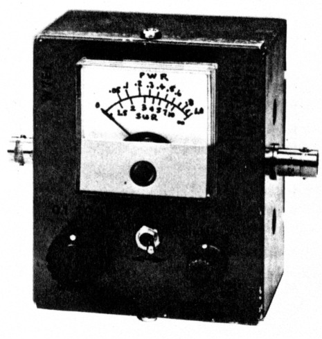
Meter face
You'll need to make new scales for the meter or, at the very least, add markings to the existing scale. It's fairly easy to make the new scales readable and somewhat harder to make them look nice. If you decide to make new scales rather than add marks to the existing scale, you'll want to record the correct places to make the new marks before you obliterate the old scale. See this month's Hints and Kinks column for one method of relabeling a meter face.
Directional coupler
This wattmeter works best if there's a constant 50-Ω impedance from the input to the output, but it's not highly critical. There are always impedance bumps at the transitions between the coax connectors and the microstripline, and a larger bump at the coupler transformer, but these bumps can be made insignificant at HF with a little effort. Only the microstripline and directional coupler are sensitive to layout, and you have considerable latitude with these components if you know the rules.
The microstripline will be the simplest circuit board you've ever made. If you've never made a PC board before, don't worry - you can't go wrong with this one. It consists simply of a single trace on one side of the board and a ground plane on the other. There are at least three ways to fabricate this board: You can stick adhesive copper tape to the non-foil side of a single-sided board, you can etch a double-sided board, or you can cut along the edges of the line with a knife and peel away the unwanted copper.
No matter which method you choose, start with a piece of 1/16-inch-thick, glass-epoxy PC board. The board's length should equal or exceed the distance between wattmeter input and output connectors, and the board should be at least one inch wide (wider is okay). The width of the microstrip, which should be about 0.1 inch, determines the im pedance of the line. Impedance doesn't change much as line width changes, and the impedance isn't too critical for this application. So if you don't have a decimal ruler, just make the trace a bit thinner than 1/8 inch - it'll be close enough. After making the board, cut a hole in the center just large enough to accommodate transformer T1. The finished microstripline should look like that shown in Fig 4.
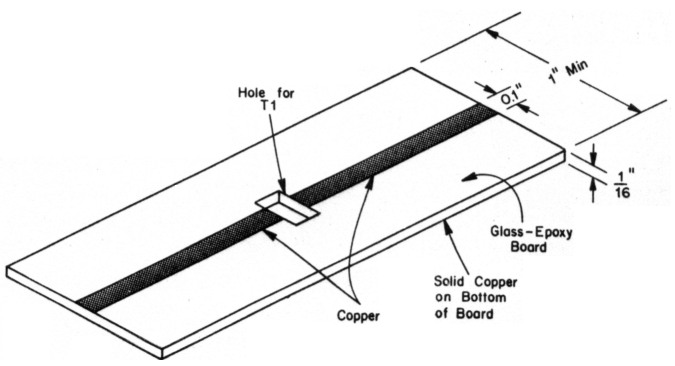
Fig 4 - Completed detector circuit board. Not drawn to scale.
Mount the coupler components using short leads. A suggested layout is shown in Fig 5. Then assemble the rest of the wattmeter and mount the completed coupler between the input and output connectors. The connections from the connectors to the microstripline must be very short, particularly the ground connections. If possible, put a elder lug or lugs on the connector-mounting screws and solder the lugs directly to the bottom of the line as shown in Fig 6.
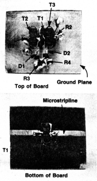
Fig 5 - Close-up views of the completed directional coupler. T1's primary is a straight piece of insulated wire spanning the cut in the microstripline. T1's secondary winding is routed through the hole cut for T1. The top view shows the components comprising the directional coupler and detector. To achieve minimum lead lengths, R1-R4 are mounted vertically on the ground plane. Capacitors C1 and C2 are not shown, although they should be mounted directly across R3 and R4, respectively.
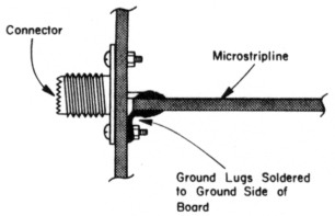
Fig 6 - Using solder lugs to make a good connection to the ground side of the microstripline.
A template package containing a PC-board pattern integrating the wattmeter circuit and directional coupler, parts-placement diagram and other information is available from the ARRL Technical Department Secretary for a no. 10 SAE with return postage for I ounce.
Tips
A small center-off toggle switch, wired for REV-OFF-FWD operation, is a convenient way to combine S1 and S2. However, small toggle switches are amazing in their ability to turn themselves on at the slightest provocation - like being bumped around in a suitcase or backpack. So if you're going to use this wattmeter for portable operation, use some other kind of switch (a slide switch, for example) for, or in series with, S1.
I've seen quite a few articles implementing the Bruene directional-coupler circuit with a powdered-iron core (eg, T-68-2). The low winding impedance of such a transformer will ruin the accuracy of this circuit, so don't use powdered-iron cores for the transformers in this wattmeter.
Adjustments
All you'll need for adjustment is a high-impedance dc voltmeter. Connect the voltmeter between the wiper of the SENSITIVITY control (R6) and ground. Connect a temporary jumper between pins 7 and 3 of U1. Turn R6 fully counterclockwise. Set the FULL SCALE SELECT switch S3 to the 10-W position. Turn on POWER switch SI. Slowly turn R6 clockwise. As you do, the wattmeter and voltmeter readings should increase. If not, turn the wattmeter off and check your wiring.
Adjust R6 for a voltmeter reading of 6.49 V, then adjust R7 so the wattmeter reads full scale. Adjust R6 for a voltmeter reading of 2.05 V, then switch S3 to the 1-W position. Adjust R8 until the wattmeter indicates full scale. Adjust R6 for a voltmeter reading of 0.649 V, then switch S3 to the 0.1-W position. Adjust R9 for a full scale reading on the wattmeter. Turn the wattmeter off and remove the temporary jumper between pins 3 and 7 of U1. This completes the calibration.
To obtain maximum reliability, measure R7, R8, and R9 and replace them with fixed resistors of the measured values; readjustment should never be necessary.
If you need to measure SWR at levels very close to 1:1, you may want to tweak the wattmeter to show a zero-reflected-power indication when connected to a reference dummy load. The resistors to adjust are R1 and R2. Theoretically, the correct value for these resistors is 49.5 Ω each. It's not necessary to readjust the wattmeter if you change the values of R1 and R2 slightly.
Use
To measure power, select the appropriate scale and turn S6 fully clockwise. The power flowing in the line is the forward reading minus the reverse reading. To measure SWR, switch S3 to the next more sensitive setting and switch S2 to FWD. Adjust R6 for a full-scale meter reading. Flip S2 to REV and read the SWR scale. To adjust a Transmatch, put the wattmeter between the transmitter and Transmatch and adjust the Transmatch for zero reflected power.
The directional wattmeter can do anything an SWR meter can do, and many things besides. Because you can measure power anywhere in a system, you can use the wattmeter to find cable and Transmatch losses, measure transmitter power, and lots of other things. You'll be surprised how often you reach for it!
Acknowledgments
Thanks to Dave Deford, KOED, for helping me reduce the mystery of ac versus dc response of a diode detector to the realm of physics, where it belongs.
While editing this article, QST Assistant Technical Editor Rus Healy, NJ2L, recognized the detector-diode-compensation method as the one presented by John Grebenkemper (see Note I). John Grebenkemper subsequently reviewed the article and made several useful suggestions, many of which have been incorporated into this article. One important consequence of John's comments is that they motivated me to model the performance of the detector/compensation combination for sine-wave inputs, during which I discovered an undesirably high sensitivity to diode saturation current, which is closely related to temperature. This resulted .....
(continued on page 36)
W7EL, Roy Lewallen.