Home - Techniek - Electronica - Radiotechniek - Radio amateur bladen - QST - The earth detunes my antenna
You know that the electrical quality of the soil beneath a horizontal antenna affects its impedance. But do you know how the resonant frequency is affected?
Recently, through computer analysis, I studied the effects of varying soil conditions on the feed-point impedances of dipole antennas over "real earth." Discovering how much the soil characteristics really affect antenna impedance was fascinating. I also found a few surprises in the information I gathered about the dipole.
Let's say we plan to install a half-wave, 80-meter dipole in our backyard. We have sufficient space to install it as a straight wire in a horizontal plane (how fortunate!). It will be at a modest height, 50 feet, and constructed with #12 copper wire. We want it to resonate at 3.75 MHz, the center of the 80/75-meter band. To find the antenna length in feet, we plug this frequency into the familiar equation for a ½-λ dipole, 468 divided by the frequency in megahertz, and come up with:
![]()
So we cut our dipole to this length, placing 62.4 feet of wire each side of the feed point. Now, by analysis, let's see if this antenna actually resonates at 3.75 MHz.
In this study I used NEC-2, an exceptional moments-method computer program. With its Sommerfeld/Norton method of determining ground interaction, NEC provides reliable impedance results for varying soil characteristics.(2) (MININEC and its derivative programs, such as ELNEC and MN, do not accommodate such impedance calculations, permitting evaluation only for free space or perfectly conducting earth.) For this antenna I used 11 segments (segment length is approximately 0.045 λ), and neglected copper wire losses.
To obtain meaningful information from any analysis of this nature, we must first establish a reference, or starting point. A logical reference here is a dipole in free space. where there are no earth effects. In practice, one could probably come close to reaching free-space conditions by locating the antenna in a desert with nothing but clean, dry sand to a depth of several dozen feet.
Results from NEC (rounded to the nearest tenth of an ohm) indicate the free-space feed-point impedance of our dipole is 67.5 -j41.8 Ω. This is not resonant; by definition, there is zero reactance at resonance. The 41.8 Ω of capacitive reactance indicates the applied frequency is below that of the antenna' s resonance. To reach resonance, we could either raise the applied frequency (to obtain a shorter wavelength and thus make the antenna electrically longer), or else make the antenna physically longer. NEC indicates that for resonance at 3.75 MHz, we must lengthen the antenna by about 2.5%, for a total length of 127.9 feet. That works out to be 479.6 + fMHZ, rather than the familiar 468. The calculated feed-point resistance for an antenna of this length with no. 12 wire is 72.2 Ω. (The 73-Ω value you see quoted so often for free space is for an infinitely thin conductor.) This free-space-resonant dipole, 127.9 feet long, will serve as our reference antenna.
Earth effects
Now let's see how the earth affects this antenna. From an analysis standpoint, the ground provides an image antenna beneath the real antenna, as far below the earth's surface as the real antenna is above it. For an antenna height of 50 feet, it is exactly the same as if we had two dipoles in free space, 100 feet apart. Mutual coupling, along with the earth's "efficiency" in creating the image antenna, affects the feed-point impedance of the true antenna. Because of mutual coupling, current flowing in the dipole induces current into the image antenna, which in turn induces current into the real dipole. Because the dipole's feed-point impedance equals the applied voltage divided by the total (incident and induced) current, you can see that a change in the induced-current corr:ponent causes a change in the antenna's impedance.
If the earth beneath the antenna were a perfect conductor. without losses, then the image antenna would be identical to the true antenna. The currents flowing in the two antennas would be of equal amplitude, but of opposite phase. The phase difference exists because there is a 180° phase shift in the lossless-earth reflection of a horizontal antenna. If the earth is imperfect (that is, real earth with dielectric losses), then the image antenna will have a lower current amplitude, and the phase shift will depart from 180°. This subject is discussed in more detail later in this article.
First let's consider our reference dipole over perfectly conducting earth, approximately equivalent to a solid sheet of copper extending an infinite distance in all directions. With regard to soil conditions, this is the opposite extreme of free space; instead of having no earth effects, now all rays that strike the earth are reflected. In practice, saltwater is quite close to a perfect conductor. We could probably come close to the same impedance conditions on dry land with a I-X-square copper screen on the ground beneath the antenna.(3)
If we install our reference antenna at 50 feet, NEC reports the resulting impedance over perfect earth to be 63.6 + j38.1 Ω. This means the earth is reflecting an inductive reactance into the antenna, and we must make it shorter to maintain resonance at 3.75 MHz. Analysis reveals the resonant length to be 125.2 feet, which works out to be 469.5 + fMHz. The feed-point resistance for this resonant length is 59.6 Ω. (Shortening the antenna to make it resonant lowers its radiation resistance slightly. We saw the same effect when we shortened our finite-diameter, free-space dipole slightly to make it resonant; its radiation resistance went from 73 to 72.2 Ω.)
Likely few amateurs have a backyard with conditions close to either extreme (a great depth of dry sand or t:n ex. 'rse of saltwater). Most of us have soil with electrical characteristics somewhere be+-veen very good and poor. Table 1, taken from The ARRL Antenna Book, defines the electrical characteristics for various types of soil. The analysis results so far indicate ... for a dipole at 50 feet over real earth. we must cut its length for resonance somewhere between 469.5 ÷ fMHz and 479.6 fMHz, depending on the soil conditions beneath the antenna. Additional NEC analysis reveals that for very good earth we should use 470.8 ÷ fMHz 472.7 ÷ fMHz for average earth, and 473.94 ÷ fMHz for poor earth. This amounts to an overall length change of about 10 inches from very good to poor earth, everything else being equal!
| Surface Type | Dielectric constant | Conductivity (S/m) | Relative quality |
|---|---|---|---|
| Fresh water | 80 | 0.001 | |
| Salt water | 81 | 5.0 | |
| Pastoral, low hills, rich soil typ Dallas, TX to Lincoln, NE areas | 20 | 0.0303 | Very good |
| Pastoral, low hills, rich soil typ OH and IL | 14 | 0.01 | |
| Flat country, marshy, densely wooded, typ LA near Mississippi River | 12 | 0.0075 | |
| Pastoral, medium hills and forestation, typ MD, PA, NY (exclusive of mountains and coastline) | 13 | 0.006 | |
| Pastoral, medium hills and forestation, heavy clay soil, typ central VA | 13 | 0.005 | Average |
| Rocky soil, steep hills, typ mountainous | 12-14 | 0.002 | Poor |
| Sandy, dry, flat, coastal | 10 | 0.002 | |
| Cities, industrial areas | 5 | 0.001 | Very Poor |
| Cities, heavy industrial areas, high buildings | 3 | 0.001 | Extremely poor |
Although that's not a whole lot of wire, according to NEC, it represents a change of 25.4 kHz in the antenna's resonant frequency, just because the soil ranges from very good to poor. Surprise! I used to think hams were joking when they told me their antennas' SWRs changed during periods of heavy rain, but now I'm not so skeptical. Fresh water, and presumably water-soaked ground, are high on the list of "good soils." An antenna that was resonated over poor earth could be detuned by the improved soil characteristics resulting from rain, and this would cause the SWR to rise. (If the SWR was 1:1 in 70-e line when the dipole was resonated, a resonance shift of 25 kHz would raise the SWR at the original frequency to about 1.2:1.)
Keep in mind that the above values apply only for a dipole height of 50 feet, which is about 0.19 λ at 3.75 MHz. Even then, those values are not exact because factors such as wire loops through the supporting end insulators, coupling to other objects in the vicinity, and so on, are not taken into account. It is not my intent here to provide cookbook values for precise dipole resonance for all possible situations, but rather to illustrate how soil conditions affect resonance of an antenna at a fixed height.
Other heights
The foregoing example shows that the earth, perfect or imperfect, reflects an inductive reactance into the antenna's feed-point impedance when the antenna is 0.19 A. high. Although interesting and illustrative, this analysis of a horizontal dipole at a fixed height provides information of rather limited value. A thorough analysis should examine both the resistance and reactance results for a range of antenna heights over various kinds of soil. So let us look further into earth effects.We have seen that the antenna at 50 feet must be shortened from the free-space resonant length to maintain resonance. Is this true for all heights? Certainly not! The mutual impedance from the image antenna changes with height, and therefore the resulting resistance and reactance at the feed point also change. At heights between approximately 0.33 and 0.6 λ, we'd have to lengthen the free-space-resonant antenna to maintain resonance. The same is true for heights between about 0.85 and 1.1 λ, and again for even greater heights. The exact heights where the shifts occur depend on the soil conditions, but for ground ranging from extremely poor to very good, the height difference is only a few feet at 3.75 MHz.
Information on feed-point resistance as a function of horizontal antenna height has been available in the literature for decades. Fig 1 shows the damped-sine-wave curve that has become familiar to many amateurs. But lacking in the literature is much information on feed-point reactance changes with height. An excellent article that touches briefly on this subject has recently been published,4 but that treatise primarily discusses feed-point resistance. To help fill the void in reactance information, I offer Fig 2, showing the feed-point reactance as a function of height and soil characteristics. Curves for three types of soil are included: very good, average and poor. For this portion of the analysis, the free-space resonant length (actually 127.892 feet) was held constant while the height and soil characteristics were varied.
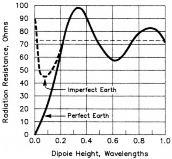
Fig 1 - Variation in feed-point resistance of a horizontal half-wave antenna at various heights above ground, after The ARRL Antenna Book (15th and 16th eds, p 3-11). The same information, less the broken line for imperfect earth, appears in Kraus (reference of Note 1, p 463).
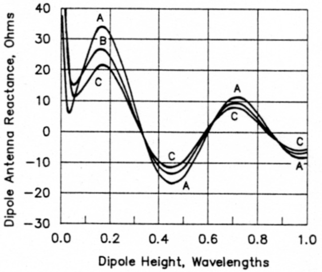
Fig 2 - Variation in feed-point reactance of a free-space-resonant horizontal half-wave antenna at various heights above imperfect ground. Curve A, very good earth; curve B, average earth and curve C, poor earth. See Table 1 for definitions of these earth types.
At first glance, the reactance curves of Fig 2 appear to resemble the resistance curve of Fig 1. But take a closer look: The peak excursions of the resistance curve do not occur at the same antenna heights as the peak excursions of the reactance curves. Instead, the zero-crossing points of the reactance curves (where the reactance goes through zero) coincide with the heights producing peak excursions in the resistance curve. And a converse situation is also true; the peak excursions of the reactance curves occur at heights where the feed-point resistance crosses 72 ohms, the resistance value for free-space.
We would expect the curve for average earth (curve B in Fig 2) to fall between curves A and C for very good and poor earth. This is indeed what happens at heights above 0.07 λ, but (surprise) does not hold true for heights below 0.07 λ. Here the reactance change with poor earth is close to that of very good earth, while that for average earth is not so close.
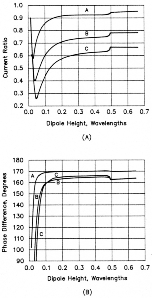
Fig 3 - Current flowing in the earth image of a ½-λ dipole over real earth versus dipole height. At A, the current magnitude is shown relative to the current flowing in the dipole itself, and at B the phase angle is shown relative to that at the dipole's feed point. For magnitude and phase, curve A is for very good earth, curve B for average earth, and curve C for poor earth. The text explains the steps in the curves.
Earth efficiency
Earlier I mentioned that the efficiency of the earth in creating the image antenna affects the actual feed-point impedance of a dipole antenna. Consider for the moment just the image antenna that exists below the earth's surface. It' s like looking into a mirror and seeing an image of yourself behind its surface. If the earth is a perfect conductor, then as stated before, the image antenna is identical to the true antenna and the ratio of the current magnitudes in the two antennas is 1:1. And as discussed earlier, there is a 180° reversal of the current phase. Again consider the mirror image. As you stand before the mirror, notice any object that exists to your left. Now consider yourself as being behind the mirror. There is a similar reversal here; that same object is now to your right, a 180° reversal.
To obtain information on earth efficiency, I treated the dipole and its image as two antennas in free space. By working from the impedances that NEC reported for the actual dipole over lossy earth, I calculated the magnitude and phase information for the current in the image antenna. (Thanks to Roy Lewallen, W7EL, for leading me to the development of a straightforward procedure to accomplish this.(5) The method is described in the Appendix.
The 1:1 current ratio and the 180° phase difference do change when the earth beneath the dipole has dielectric losses. The situation is complex, but this broad generalization states it fairly well: With the antenna at a fixed height above 0.05 λ, the current magnitude in the image antenna decreases with poorer earth. There is no surprise here; we would expect that increasing earth losses reduce the current.
The biggest surprise of this whole study came when I examined the current magnitudes in the image antenna. Without giving it really serious thought, I had always assumed that the current decreased somewhat linearly with greater antenna heights. But not so, according to calculations based on NEC results! Above 0.05 λ, the current amplitude rises logarithmically with antenna height.
I also expected the phase difference to change with height, but the results show that the phase angle remains almost constant at heights above 0.1 λ. (But magnitude and phase vary with different soil types.) Fig 3 shows the image-antenna current changes versus height for various types of soil. I did not carry the study to heights above 0.65 λ.
Refer to Fig 3A. For a given height, the current magnitudes for poor earth (curve C) are approximately 65% of that for very good earth (curve A), while for average earth (curve B) they are approximately 80% of that for very good earth. Depending on antenna height, very good earth falls in the 90% to 95% range of that for perfect earth (a constant ratio of 1.0 for all heights).
The phase angle of the image-antenna current, Fig 3B, does not change appreciably with changes in antenna height except below 0.1 λ. Rather, it depends primarily on the dielectric characteristics of the earth. For very good earth, the values hover around 170, and 165 for average and poor earth.
All the curves of Fig 3 show steps at a height just below 0.5 λ. NEC actually switches from the Sommerfeld integration method to the Norton approximation when the antenna and its image are 0.95 λ apart. The steps in the curves result from this switch at a corresponding dipole height of 0.475 λ; small discontinuities in the dipole impedances are magnified in the current analysis.
Frequency effects
The curves of Figs 2 and 3 result from using a frequency of 3.75 MHz. For a given type of soil, earth losses become greater as the frequency increases. For frequencies higher than 3.75 MHz, the curves of Fig 2 therefore exaggerate the amount of antenna reactance. Stated another way, the peak excursions for a given type of soil diminish with increasing frequency.
Additional NEC calculations disclose that, for the same electrical heights, average earth at 14 MHz produces a curve very close to curve C in Fig 2 (poor earth at 3.75 MHz). The greatest departure is for a height of 0.08 λ. where the 14-MHz curve dips to about +9 Ω reactance before rising to join curves B and C.
One thing to keep in mind concerning frequency effects is that, for a fixed physical antenna height, increasing the frequency also increases the electrical antenna height. And as an antenna is raised to greater electrical heights, the earth effects diminish. So there is a counteracting effect: higher dielectric losses from increased frequency, but lower dielectric losses because of increased electrical height. The height increase wins out; from an impedance standpoint, over real earth, the net effect is less change at the higher frequencies. Stated another way, for a fixed physical height over imperfect earth, a dipole antenna that's pruned to resonance will be closer percentage-wise to its freespace-resonant length at the higher frequencies.
Why isn't reactance information of this nature widely available in the literature? Perhaps because it is not of great consequence. Suppose you do put up an antenna and find that it's not resonant. It's generally a small task to prune the antenna to resonance, and you don't need reactance curves to aid the process. But on the other hand, you have very little control over the feed-point resistance; you must take what you get (discounting small changes with length adjustment), so resistance information is worth having for reference, to facilitate matching and the like.
So of what practical value is all this information? For one thing, this study emphasizes why the familiar dipole length equation, 468 ÷ fMHz, is presented in the texts as only approximate. Use it only as a starting point. This study has shown that with only a few height exceptions, the antenna will need to be pruned - made either longer or shorter - for exact resonance. This information may give you an idea of which way you'll need to go to adjust your antenna length, longer or shorter, for its height. It might even be possible for the enterprising amateur to gain an idea of the type of soil under his antenna by judicious use of these data. My hope, though, is that from this information you'll gain a better idea of how the earth really does detune your horizontal antenna.
Notes
- See J. D. Kraus, Antennas, second edition (New York: McGraw-Hill, 1988), pp 384-397, for a discussion of moments-method analyses.
- K. A. Norton, The Propagation of Radio Waves Over the Surface of the Earth and in the Upper Atmosphere," Proceedings of the IRE, Vol 26, #9, Sep 1937, and A. Sommerfeld, Partial Differential Equations in Physics (New York: Academic Press, 1964). The Sommerfeld/Norton NEC option uses a numerical evaluation of the Sommerfeld integrals for ground fields when the interaction distance is below 1 X, and uses Norton's asymptotic approximations for larger distances.
- Although a reflector screen as described in the text may provide impedance conditions similar to perfect earth, it could not provide the same far-field radiation pattern or the same gain from earth reflections. To obtain equivalent far-field performance, the screen would require a radius of approximately 15 to 20 k, depending on antenna height.
- C. Michaels, W7XC, "Dipoles above Real Earth," Technical Correspondence, DST, Nov 1992, pp 67-68. Also see Feedback in the January and February 1993 issues.
- Private communication. The method I used assumes uniform sinusoidal current distribution in both antennas, a situation that may not be precisely true in reality.
- See the referent of Note 1, p 463.
Appendix
The analysis of the current ratios as graphed in Fig 3 is based on the relationship from Kraus:(6)
![]()
where all terms are complex, and where
V1 = the applied voltage at the dipole antenna terminals
I1 = the dipole antenna current
I2 = the image antenna current
Z11 = the self-impedance of the dipole in free space
Zm = the mutual impedance between the dipole and its image at a spacing of twice the dipole height
From this relationship,
![]()
where Z1 is the dipole impedance above real earth (as calculated by NEC). Rearranging terms, the relationship becomes.
![]()
Remember, all the terms in each of these equations are complex, with a real and an imaginary component (such as R + jX for an impedance.)
Mutual impedance and mutual coupling are discussed in Chapter 8 of The ARRL Antenna Book, 15th and 16th editions (1988 and 1991), p 8-4. Also see the Antenna Book's Fig 19 for a graph of mutual resistance and reactance values versus spacing.
To verify the results of this technique, I used ELNEC to calculate and plot the broadside elevation patterns of a half-wave dipole at several heights above real earth. Then I calculated and plotted the impedances and patterns for the dipole and its image as an array in free space, with element separations of twice the various heights. For each height I set the element current ratios at the magnitude and phase angle determined from Eq 3. The impedances of the upper element in the free-space array (the "dipole") reported by ELNEC agree well with the impedances NEC reports for a dipole over real earth.
The patterns also agree well. A comparison of one pair of patterns from the two calculations is given in Fig 4. The patterns over real earth contain a theoretical 3 dB gain from earth reflectivity (the dipole pattern is contained in only the upper hemisphere, whereas the array in free space is not limited in this way). Otherwise the patterns compare very favorably. The excellent agreement of the dipole impedances and patterns indicates that this method of current analysis is valid.
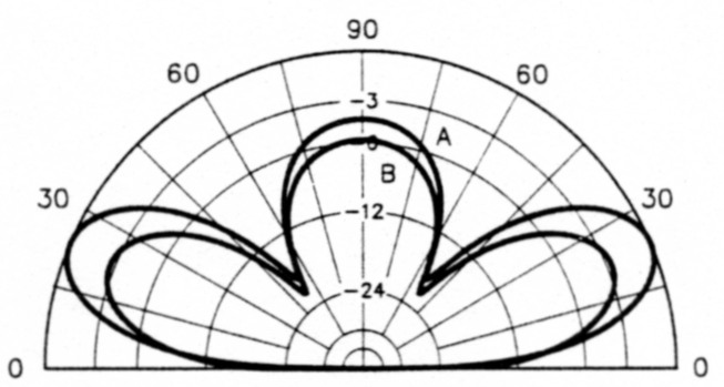
Fig 4 - Elevation-plane radiation patterns calculated with ELNEC. Curve A, the pattern of a 0.6-λ-high dipole over average earth (see Table 1) at 3.75 MHz. Curve B, the pattern of an array of two dipole elements in free space, 1.2 λ apart, and using a phase difference determined from Eq 3. This array represents the dipole and its earth image. In theory, Curve A should exhibit 3 dB more gain at all angles because of earth reflectivity, but earth losses reduce that value. Here the difference at 23° is 2.6 dB, and at 90° is 1.5 dB. The favorable NEC and ELNEC comparison of the patterns and feed-point impedances at this and other heights indicates the current analysis method of the Appendix is sound.
K1TD, Jerry Hall.