Home - Techniek - Electronica - Radiotechniek - Radio amateur bladen - QST - Mother nature's radio
Despite our modern understanding of radio phenomena, the study of the Earth's natural VLF radio emissions is hardly out of its infancy. The best part is - you can get involved!
The Sounds of Natural VLF Radio
As the Earth races on its complicated path through the heavens, powerful and mysterious planetary forces work their magic. The result: a cacophony of "natural radio" sounds:
Chorus: Chorus sounds like a flock of chirping birds! It occurs most frequently in the morning hours, hence its nickname "dawn chorus." Increasing tones between 1 and 5 kHz seem to be most common. Chorus is usually accompanied by other VLF phenomenon such as hiss or whistlers.
Hiss: Hiss sounds just like its name. A continuous band of frequencies denotes VLF hiss. Sonograms of hiss signals have shown cutoff frequencies ranging from 2 to 30 kHz. Hiss has also been associated with enhancements in auroral activity.
Tweeks: Tweeks are believed to result from "spherics" that echo back and forth in the Earth-ionosphere waveguide. They usually sound pure in tone, much like a note from a musical instrument. The tone sometimes resembles a "ping" sound.
Whistlers: Whistlers tend to be most common at night or just before dawn. They are also more frequent at mid-latitudes, peaking between 40-55 degrees geomagnetic latitude. See the text for more details.
If Mother Nature had made our ears capable of hearing electromagnetic radiation instead of audible sounds - in our normal auditory hearing range of 20 Hz-20 kHz - what could we hear? As it turns out, a lot! We'd hear "chorus," "hiss," "tweeks," "whistlers" and other exotic sounds. See the sidebar, "The Sounds of Natural VLF Radio."
What are these sounds and where do they come from? They're natural sounds generated in the audio-frequency range of the electromagnetic spectrum. The audio-frequency range of the spectrum covers the same range of frequencies as the audio-frequency (sound) portion, but electromagnetic waves travel at the speed of light, not at the speed of sound. In other words, our ears can hear a 10-kHz audio sound, but we can't hear a 10-kHz electromagnetic (radio) wave unless it's electronically converted to an audible sound (hence the need for radio receivers!).
These sounds are associated with disturbances in the Earth's atmosphere. They're initiated by lightning and by the charging of the atmosphere by the Sun.(1) The frequencies that produce these unusual sounds reside, for the most part, between a few hertz and several hundred kilohertz.
This broad range of frequencies is broken down into three main segments (see Table 1). Most of the naturally occurring radio effects from lightning have a maxi mum frequency of about 5 kHz, so these sounds usually fall into the Very Low Frequency (VLF) part of the electromagnetic spectrum.
| Description | Abbreviation | Frequency | Wavelength |
|---|---|---|---|
| Extremely Low Frequency | ELF | 3 Hz-3 kHz | 100,000-100 km |
| Very Low Frequency | VLF | 3-30 kHz | 100-10 km |
| Low Frequency | LF | 30-300 kHz | 10-1 km |
HF-and-higher frequencies refract through the ionosphere, allowing communication over great distances. The lower ionosphere, the D layer, is about 80 km above the surface of the Earth. This means that about 4000 full waves at 20 meters (14 MHz) can fit between the Earth and the lowest layer of the ionosphere.
At VLF, however, only a few waves (or a fraction of a wave) can fit in this space. For example, a 5 kHz VLF signal has a wavelength of 60 km - it's barely able to fit in the D-layer waveguide! (The D-layer waveguide, or the Earth-ionosphere waveguide, are terms that describe the 80 km space between the surface of the Earth and the bottom of the D-layer.)
Armed with this knowledge, you'd probably think that naturally occurring VLF radio waves travel only short distances, at least by conventional propagation.
Well, by more conventional propagation modes, VLF signals do travel relatively short distances, but even early experimenters proved that VLF waves can traverse large distances.(1) In fact, VLF waves can travel from one hemisphere to the other and back again!
Although HF radio waves sometimes travel thousands of miles from transmitting antenna to receiving antenna, VLF radio waves can travel more than 100,000 miles from a lightning stroke to a receiving antenna. The mechanism that propagates these VLF waves isn't the more-familiar ionosphere, it's the Earth's magnetosphere.
Planetary magnetospheres resemble magnetic dipole fields, but their currents flow in the plasmas that extend from the outer ionosphere to thousands of miles in space. These currents, resembling the familiar horseshoe-shaped magnetic flux lines, result in part from solar winds that reach the Earth and from the rotation of the Earth about its axis.
A wealth of information can be gained from the study of natural VLF waves. Propagation information, electron densities in the ionosphere and magnetosphere and the location of the lightning strikes that cause particular VLF waves are a few of the studies that are under way.
Man-made VLF signals are exploited by several groups, especially the US Navy. The Omega signals broadcast at various places around the Earth are used as maritime and aviation navigation aids. Manmade VLF generally falls in the 10-40 kHz range. These predictable signals can be used in conjunction with naturally occurring VLF to help us better understand their propagation characteristics.
Whistler VLF Theory
Whistlers are interesting and informative natural VLF radio waves (see Fig 1). A whistler is a VLF wave that originates with a lightning strike. Generally, there are at least two wave events associated with the lightning pulse. The first event is a short-lived wave that propagates from the lightning strike through the Earth-ionosphere waveguide to the receiver. This event is called the atmospheric, or simply spheric.
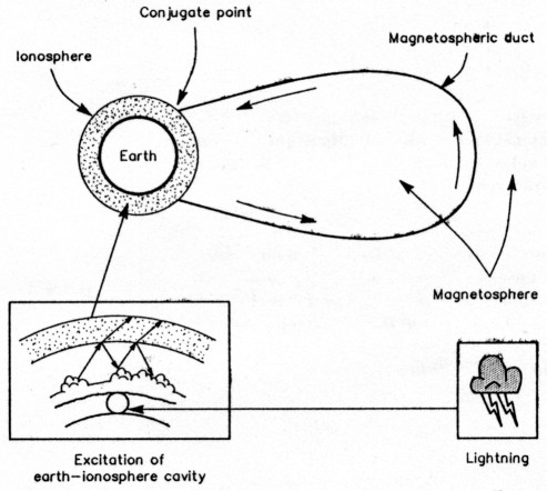
Fig 1 - Schematic showing the generation and propagation of ducted whistlers.
The second event is the whistler itself. The whistler wave travels up to and through the ionosphere, enters the magnetosphere and follows the Earth's magnetic field through a relatively narrow magnetic "duct" to the opposite hemisphere. After arriving in the opposite hemisphere, it again traverses the ionosphere, exits and propagates in the Earth-ionosphere wave-guide to the receiver.
This is called a "one-hop" whistler; you can see the reason for its delay time relative to the spheric. A "two-hop" whistler is one in which the hemisphere where the lightning stroke originated also receives the whistler wave after it's ducted twice in the magnetosphere.
Under the right atmospheric conditions, this "hopping" between hemispheres can happen many times, sometimes several hundred! The number of hops determines the delay between the lightning strike that produces the original spheric and the whistler event.
Ducts that direct the whistler wave to the opposite hemisphere end up at a conjugate point on the Earth's magnetic field. A whistler that originates in the Northern Hemisphere will be ducted to the Southern Hemisphere to a point in the Earth's magnetic field equal in magnitude to the magnetic field where it originated.
The physical consequence of traveling thousands of miles through magnetic ducts is that higher frequencies arrive at the receiver before the lower frequencies (see Fig 2). The more hops the whistler takes, the greater the time between the higher- and lower-frequency arrivals (that is, the dispersion increases).
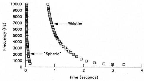
Fig 2 - A lightning "spheric" followed by a "ducted" whistler.
An accurate measurement of the dispersion can lead to an understanding of the whistler's propagation path, as well as the whistler's spectral shape. In addition to being fun to listen to, a deeper understanding of the composition of the ionosphere and the magnetosphere (ion density, electron density, electron temperature, and so on) can be realized.
How to Get Involved in Whistler Research
Hams took part in receiving natural VLF signals across North America this past year, and you can participate in this monitoring program and directly contribute to scientific endeavors of great interest to NASA, the Navy and the scientific community.
Further analysis of whistlers and their sonograms is ongoing. Northern Kentucky University and VLF monitoring teams across North America will make additional recordings in March 1994.
Our goal is to expand our efforts to other parts of the globe and incorporate VLF recordings from as many different geomagnetic locations as possible. If you'd like to take part in this scientific team effort, please write me at the address shown at the beginning of this article. We'd like to hear from you!
Whistler VLF Experiment
One way to study whistler phenomena is to simultaneously record whistlers at sites hundreds or even thousands of miles apart. This technique can provide information on whistler propagation by directly comparing the spectra of the same whistler recorded simultaneously at distant sites.
For example, a one-hop whistler must traverse the ionosphere at least twice and enter at one place into the ionosphere from the magnetosphere. By comparing the spectra of the same whistler at receiving stations thousands of miles apart, we can look for changes in the wave form.
This may manifest itself in one spectra as a missing or attenuated segment that may be caused by absorption as the whistler wave travels from its exit point in the ionosphere to a distant receiver.
Noting which frequency components have been attenuated can lead to information about which part of the ionosphere-the D, E or F region-caused the effect. As you may guess, receiving a whistler that has propagated through the gray line-the line separating day from night-could give details about the density of ions and electrons in the D region, which is most pronounced on the daylight side of the Earth.
Fig 3 shows a schematic for a typical VLF monitoring and analysis station. The basic configuration consists of the VLF receiver and antenna, a timing device (usually WWV's 5, 10,15 or 20-MHz time signal broadcast from Ft Collins, Colorado) and a stereo cassette or VHS recorder.
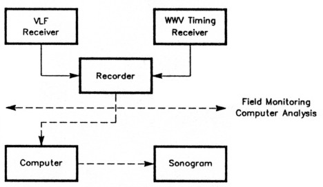
Fig 3 - A typical whistler recording and analysis setup.
One channel of the stereo recorder will record WWV, and the other channel will record the natural VLF phenomenon. Using a single timing source makes it possible to accurately compare recordings made simultaneously at several locations.
VLF receivers can be purchased from Conversion Research for about $70 (complete with an antenna), or you can make one from inexpensive parts.(2) Computer analysis can then be accomplished with commercial software and hardware, such as Sound Edit and Mac Recorder on an Apple Macintosh computer. Display and analysis of sonograms can also be done with counterpart software on an IBM-compatible PC.
Whistler sonograms recorded March 22, 1993, are shown in Fig 4. These sonograms, recorded at several points in North America, are of the same whistler. The horizontal lines near 10 kHz are man-made Omega broadcasts. The vertical lines are spherics from local lightning discharges. The variation in cutoff frequencies for this whistler at various locations provides clues to its propagation characteristics in the Earth-ionosphere waveguide.
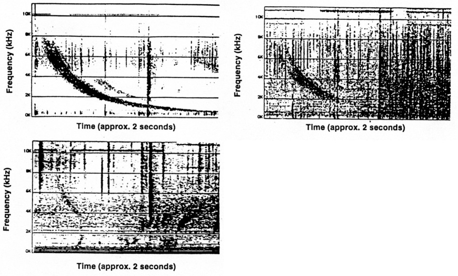
Fig 4 - Sonograms of whistlers recorded in North America.
Acknowledgments
The success of this VLF program is possible because of dedicated participants at Northern Kentucky University and across the US. Contributors include Dr Mike McPherson, Dr Bill Wagner, Dan Spence, Toxanne Barnes, Steve Phelps and Justin Rains. Special thanks goes to Dr Dennis Gallagher of the Magnetospheric Physics Branch of NASA's Marshall Space Flight Center.
Funding for the VLF project is provided by the Kentucky Space Grant Consortium (KSGC) and NASA.
Notes
- See, for example, R. A. Helliwell, Whistlers and Related Ionospheric Phenomena, Stanford University Press, Stanford, California (1965).
- An excellent description of whistlers and other VLF phenomenon, plus instructions on how to build a VLF receiver, can be found in the July 1992 issue of Science PROBE! The article is titled "Listening to Nature's Radio," by Michael Mideke.
AD4CC, David Schneider.