Scope that signal
Are you overmodulating? Is your linear linear? Find out with a station monitor you've built from scratch.
Do you worry? I do. When I operated SSB, I always used to worry about whether my rig was adjusted properly to put out the best possible signal. My rig, like many transceivers today, uses a linear stage for the final amplifier regardless of the mode of operation, be it SSB or CW, and the only intrumentation provided is the ubiquitous panel meter. In addition, I had a directional coupler for measuring forward power and vswr. With this arrangement; tuning up for CW is no particular problem: Just put the key down, keep the plate current more or less dipped (it's a vacuum-tube final), watch the forward-power meter, and tune for maximum smoke (that is, forward power: while not exceeding a certain maximum allowable value of plate current.
With SSB (and to a lesser extent AM, assuming there is anybody out there still running AM) the problem is not so easy, however. Since panel meters can't respond to the instantaneous changes in the transmitter during modulation, an oscilloscope must be used for monitoring the true state of the transmitted signal. Some fine monitor scopes designed specifically for amateur use are available commercially, but the prices are rather steep. Consequently, most of us fall back on the time-honored procedure of setting the rig to the Tune position, putting out a single CW note, and tuning for maximum forward power. When the rig is switched back for SSB modulation, we just hope everything will come out OK. Nevertheless, this still leaves unanswered the question of whether the rig is properly tuned up. Being the sort who worries endlessly about such little questions, I used to sit there and worry.
This state of affairs persisted up until August, 1983, when the FCC finally changed the rules on maximum allowable power for the Amateur Radio Service. Whereas previously we were limited to 1-kW-dc input power with no limit on output power, now we have a 1500-Watt limit on PEP output power with no limit on dc input power (except for AM DSB which temporarily remains unchanged). In order to most effectively utilize the new rule, we now need the ability to make accurate output-power measurements for all modes of operation. An oscilloscope nicely meets this requirement. Consequently, I finally came to the decision that I had to have a monitor scope. With the prices of the commercial units making them out of the question for me, I would have to build one.
What follows is a description of a monitor scope that is relatively easy to build and that is cheap. The whole cost was less than $50.00, exclusive of the price of the CRT (which was already on hand, having been obtained -many years previously by a method so unlikely as to be quite unbelievable). The device includes a built-in two-tone signal generator and a two-speed linear-sweep generator, one sweep speed being used for examining the two-tone test pattern (or just a single-tone pattern for AM rigs) and the other speed being used for examining voice patterns during normal station operation.
While most readers will not wish to duplicate the Unit in its entirety (especially the toroidal transformer for the horizontal-sweep volt-'age), the main circuitry is so straightforward that it should serve as an excellent starting point for those wishing to build their own monitor scope. Those who already have a general-purpose oscilloscope equipped with an external input to the horizontal amplifier (which also provides, or can be adapted to provide, a direct connection to the CRT vertical-deflection plates) will need to build only the main circuitry and the low-voltage power supplies to obtain a first-class scope.
General Description
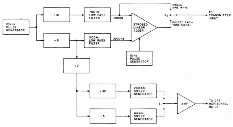
Fig 1: Block diagram
Fig. 1 is a block diagram of the monitor which illustrates the key features of the unit. A 12-kHz pulse generator is the initial source for each of the two sine waves used for the two-tone signal (1200 Hz and 2000 Hz) and it also is the source for the trigger pulses for the CRT sweep waveform. The 1200-Hz sine wave is derived by digitally dividing the 12-kHz pulses symmetrically by ten, and then passing the resulting square wave through a 700-Hz low-pass active filter. The 2000-Hz sine wave is similarly derived, except that the division is by six and the low-pass filter has a cutoff frequency of 1100 Hz.
The two sine waves are then linearly added in a strobed adder circuit driven by a separate asynchronous pulse generator running at about 10 Hz. By adjusting the duty cycle of the asynchronous pulse generator to approximately 33%, the re-suiting pulsed two-tone test signal can be continuously applied to the transmitter under test without exceeding the transmitter's maximum dissipation limits. At the same time, the CRT display appears to be continuous and can be examined at your leisure. While the trick of pulsing the two-tone test signal is not new,(1)(2) its use has not appeared in the literature for a long while; it is a technique worth remembering. Provision is also made for running the adder continuously; in this manner the PEP dc input power may more easily be determined (see below).
Besides generating a two-tone test signal, the monitor also can provide just the 1200-Hz sine wave as a test signal for use with AM rigs. Since AM transmitters must have sufficient dissipation capability to run with continuous modulation, the 1200-Hz signal need not be pulsed.
In addition to the sine waves, the trigger pulses for the sweep generators are also derived by digital division. The 2000-Hz square waves are further divided by ten to provide 200-Hz pulses for triggering the 4-ms sweep generator, and by 60 to provide 33-1/3-Hz pulses for triggering the 24-ms sweep generator. The 4-ms sweep displays 3.2 complete beats of the 800-Hz difference between the two sine waves, while the 24-ms sweep is a convenient speed for viewing voice patterns.
It is important to note that by this choice of division factors (2, 5, and 6), the 4-ms-sweep repetition rate of 20G Hz is an exact submultiple of both of the sine waves; and since all three waveforms are derived by digital division of one common oscillator, the relative phases of the three waveforms are fixed and cannot change even if the 12-kHz oscillator drifts in frequency. In this manner an unconditionally-stable CRT display is produced without the complication of involved level-sensitive trigger circuits such as are found in the normal measurement oscilloscope. The 24-ms-sweep divisor chain, while mainly intended for voice-pattern observation, also contains the same division factors; it, too, will produce a stable two-tone pattern if desired. Similarly-stable AM-envelope test patterns are also produced.
Main Circuit
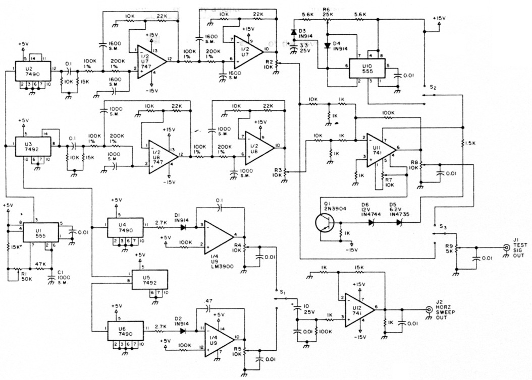
Fig. 2. Main circuitry.
The main circuitry which forms the heart of the monitor scope is shown in Fig. 2. A 555 timer, U1, is the 12-kHz pulse generator, with R1 providing fine frequency adjustment. The exact values shown need not be used, but all resistances and the value of the timing capacitor, Cl, must be changed proportionally if the 12-kHz oscillation frequency is to be maintained. Although drift in the oscillator frequency will not cause the CRT display to change, a capacitor with good stability, such as a silvered mica or a polycarbonate, should be used at C1.
U1 directly drives the di' vider chain of U2 through U6. Initially, regular TTL packages were used, but the current consumption was over 150 mA, which proved to be a little too much for . the heat sink used on the +5-V-dc regulator. Low-power Schottky devices were substituted and the current consumption dropped to around 65 mA.
The 1200-Hz square waves from U2 are applied to the input of the 700-Hz, two-stage, active low-pass filter formed by U7, while the 2000-Hz square waves from U3 are fed to the 1100-Hz filter formed by U8. In this case, type-747 packages (dual 741s) were used, but individual 741s may be used if desired (or a single LM348 quad 741s can be used if obtainable). Both of the filters are implemented using the op amps as non-inverting voltage-controlled voltage sources with a passband gain of two (set by the 10k and 22k resistors). By picking the gain to be two and using equal values for the two frequency-determining capacitors in each stage, the formulae for the required resistances simplify to R1 = Q/(2irfC) and R2 = R1/Q2, where R1 is the input resistor (100k) and R2 is the resistor between the two capacitors (200k). The Q of the filters was set at 0.707 to prevent ringing.
Again, there is nothing sacred about the exact values used, and the ones shown here were picked entirely as a matter of convenience from parts on hand in the junk box. Thus the gain-setting resistors could just as easily have been 4.7k and 10k, or 22k and 47k, etc. If a capacitance value other than 1600 pF is desired, the 100k and 200k 1% resistors can be replaced according to the formulae above. However, resistance values much larger than the 200k shown here should be avoided to prevent difficulties caused by the op amp's input offset currents. Although 1% resistors are shown, 5% values can probably be used in the filters without any serious loss in performance.
The recovered sine waves from the low-pass filters are linearly added in U11. A package with a single op amp is required here to allow strobing. Stage gain is set for 100 to prevent an objectionable amount of signal feedthrough when power is not applied to the adder. The signal level out of the low-pass filters is about 1 volt peak. To prevent saturation of the adder, the level-setting pots, R2 and R3, attenuate the tones by a factor of ten; a further reduction is achieved by the 10-to-1 dividers between the pots and the input to the adder.
The 10k pot, R8, on the output of the adder allows the two-tone signal to be attenuated to the level of the 1200-Hz sine wave so that if you want to switch between the two-tone signal and the 1200-Hz sine wave when testing, the signal level to the transmitter remains the same. Either the two-tone signal or the straight 1200-Hz sine wave is selected by S3, and the level to the transmitter is set by R9.
A second 555 timer is used for the asynchronous 10-Hz pulse generator that provides the strobed power for the adder; either these pulses or continuous power may be selected by S2. Use of the two blocking diodes, D3 and D4, divorces the charging-current path from the discharge-current path to allow duty cycles less than 50%. Equalizing zener diodes D5 and D6 provides the base drive for the V-strobe transistor, Q1, or a single zener in the 18-to-24volt range could be used if available.
Two separate CRT sweep generators were built, each using 1/4th of an LM3900 package with the sweep speed being selected by S1 (the remaining two quarters were not used). Sweep time is determined by the capacitors, and it was felt that it was best not to put the selection switch in the capacitor circuit. Since the LM3900 operates from a single-ended supply, the sweep voltage is always positive and a blocking capacitor has to be used before the following amplifier to remove the dc component of the sweep waveform.
The leading edge of the trigger pulse from the divider chain sets the generator output low, and then the output starts rising .linearly as soon as the trigger pulse goes low. The output continues to rise until maximum supply voltage is reached, at which point the generator locks up until the next trigger pulse resets it.
Consequently, to produce a linear sweep with no high-level dead time, the interval between trigger pulses must be less than the maximum available charging time for the capacitor. As long as this criterion is met, sweep time will be determined by the interval between trigger pulses and not by the value of the capacitor, per se. However, if the maximum available charging time is very much longer than the interval between trigger pulses, relatively little sweep voltage will be developed. Hence, for a given trigger-pulse interval, some reasonable capacitor value must be chosen. The values shown are about optimum for the trigger pulses used here, and the sweep-generator outputs are each about two volts peak. Equalization of CRT sweep widths are obtained with R4 and R5, and a sweep output of about 20 volts peak is produced by the U12 amplifier stage following the generators.
As mentioned previously, the circuit of Fig. 2 is all you'll need if you already have a general-purpose oscilloscope that has its own built-in horizontal amplifier and direct access to the vertical plates. If you fall into that category, you can skip the next section and go look at the power supplies. But if you want to start from scratch with just a CRT, the next section will show you how to do it.
CRT Circuit
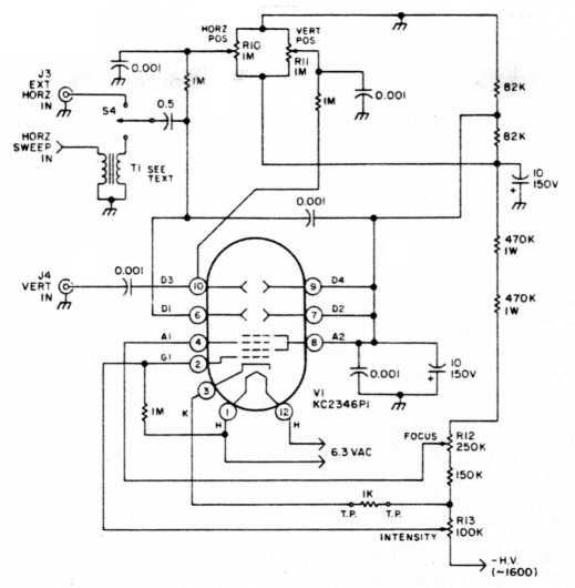
Fig. 3. CRT circuitry.
In Fig. 3 you can see what's needed to hook up a CRT to get a usable trace. It's a simple circuit and is basically taken straight from any copy of The Radio Amateur's Handbook between 1%2 and 1980. (I presume it's in later editions also.) All resistances are 10%, and all wattages are 1/2 Watt, except for the two 470k, 1-W resistors. There are a few changes from the basic Handbook circuit that are worth noting here.
Since the high-voltage supply I. built provided 1600 volts, the voltage divider chain was adjusted to draw 1 mA at this voltage. I then picked the 100k and 250k pots and the 150k dropping resistor to roughly match the recommended range of operating voltages specified by the data sheet for the DuMont KC2346P1 CRT. This tube has a deflection sensitivity of about 25 to 30 volts per inch, so the 82 volts of plus-or-minus dc voltage on the plates guaranteed that the trace could be moved anywhere on the face of the screen. I'll give you 100-to-1 odds that you won't be using this particular CRT, but the adjustment range can easily be changed by altering the 82k resistors for any CRT you happen to have.
Don't forget to include the 1-M resistor that ties the heater to C1. Most CRTs aren't built to have more than about 150 volts be tween cathode and heater. You can run the resistor to the cathode instead of G1 if it's more convenient with your particular tube.
You will also note a .001-uF disc ceramic across the horizontal-deflection plates. This capacitor helps keep rf off these plates, and it will help extend the usable upper frequency limit of the CRT. Mount the capacitor on the CRT socket directly between the terminals for the horizontal plates to get the maximum possible benefit.
The 1k resistor, in series with the cathode, is used to measure beam current to verify that you are not drawing excessive current from the electron gun. The current is determined by carefully measuring the voltage drop across the resistor. Be extremely careful if you do this, because the whole meter and its leads will float up to almost the full value of the high-voltage supply. A shock from a 1600-volt supply is always a very serious matter, if not a fatal one.
Now comes the problem of how to get the necessary horizontal-deflection voltage to sweep the CRT. The DuMont tube was a three-inch tube, so it required something like 100 volts of sawtooth to sweep it. Some of the older and more common CRTs, like a 3AP1 or a 5BP1, have deflection sensitivities as low as 150 volts per inch, or worse. With one of these tubes, 500 or more volts of sawtooth might be needed. Sweep voltages of this magnitude are difficult to produce with common solid-state components-and besides, I didn't want to include yet another supply in the monitor. So instead I built the sweep transformer, T1, winding it on an Amidon FT-193-J toroidal ferrite core.(5)
Without going into the theory of transformer design, I want to point out two requirements that had to be met: First, there had to be enough turns on the primary to avoid saturating the core, and second, the self-inductance.of the primary had to be high enough to present a reasonably high impedence to the driving source. After a great deal of fiddling around, I determined that with this core, 200 turns on the primary would be enough for the fast sweep speed, so when I wound it, I ised 300 turns to be safe.
For the secondary, I used 4500 turns to obtain a 15-to-1 step-up transformer. Since the U12 amplifier stage put out about 20 volts, I ended up with about 300 volts of peak sawtooth which was more than enough for the DuMont tube. However, at he slow sweep speed the core would saturate before a full-screen sweep could be obtained, so I had to limit myself to about 2.5" of deflection for voice patterns. Probably 400 turns on the primary and 6000 turns on the secondary would have been a better choice for this core.
Let me hasten to add that I had access to a toroidal-coil winding machine and I did not wind T1 by hand. Amidon now offers ferrite E cores which come in two halves, and with these cores a bobbin can be wound normally using an electric drill. This is a much more practical procedure for home construction. For anyone wishing to try an E core, I would recommend using one of the larger sizes rated for 100 to 200 Watts when used as a power transformer.
Another way to obtain the sweep voltage, of course, is to build a several-hundredvolt supply and use a vacuum-tube amplifier to develop the sweep voltage.
However the sweep voltage is obtained, provision should also be made for an external horizontal input to enable production of the trapezoidal pattern when checking AM rigs.
Power Supplies
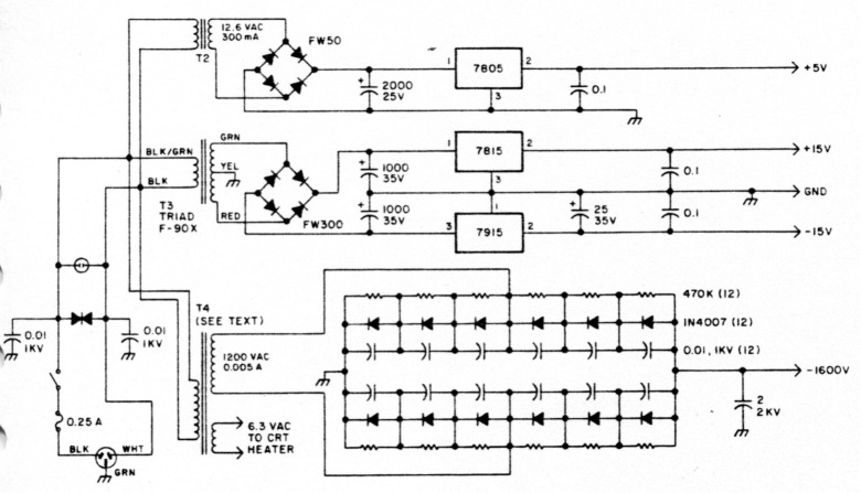
Fig. 4. Power supplies.
Construction
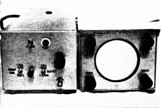
Photo A. The monitor scope is built in two enclosures. The one on the left contains the power supplies and the main circuitry.
Construction of the monitor scope is straightforward as shown in Photo A, the unit was assembled in two separate enclosures, one for the CRT and its associated circuitry of Fig. 3, and a second one for the remainder of the circuitry. The two enclosures were connected by a heavily-shielded cable. In this manner, the CRT was kept far away from the stray fields of the power transformers which otherwise could have blurred the oscilloscope trace. Point-to-point wiring was used in the CRT gnclosure, while perfboard construction was used in the other. All ICs, U1 to U12, were mounted with sockets on the perfboard.
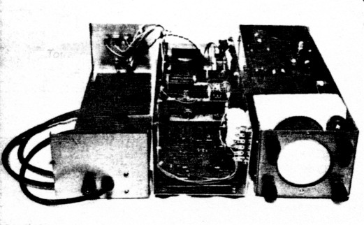
Photo B. Interior view of the monitor scope. The power supplies are at the rear.
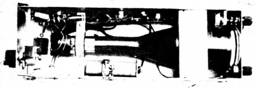
Photo C. Details of the CRT mounting. Note the clamps on the neck and the styrofoam block on the body of the CRT.
Mounting the CRT is a little tricky because of its fragility. The method used here is shown in Photos B and C. A screen was made of hard clear plastic by inscribing a centimeter graticule with a ruler and a sharp point. This screen was placed directly inside the enclosure over the opening for the CRT face. The face of the CRT was placed against the screen, and the CRT was supported on its large front diameter by cutting a tight-fitting hole for the CRT in a block of styrofoam that was in turn fitted to the inside enclosure.
The neck of the CRT was captured and supported by two V-brackets made of aluminum strip. The brackets clamped the neck of the tube from above and below. Before clamping, a piece of rubber from an inner tube was placed around the CRT neck to prevent direct metal-to-glass contact. In this manner, the neck could be gripped quite securely without damage.
Special care in mounting was also needed for potentiometers R12 and R13, the focus and intensity adjustments, respectively: As can be seen in Fig. 3, these controls float at high voltage. They were mounted on a small piece of hard plastic, and insulating couplings were used to couple the shafts tc the knobs on the outside.
No other additional precautions have to be taken other than to use good engineering practice when wiring the CRT HV supply, and to use leads as short as possible for bringing the rf to the hot CRT vertical-deflection plate.
Adjustment and Checkout
If a general-purpose oscilloscope is available, it will be very useful for checking the operation of the main circuitry (although you can get by without one). If you can borrow one for the adjustment, it will be worth the effort.
Build the power supplies and get them working first; then start on the main circuitry. I found it useful to build one -functional block at a time and check it out before I went on to the next. This method seems to make troubleshooting easier. If some method of checking frequency is available (e.g., a calibrated oscilloscope), adjust R1 to produce 12-kHz pulses from U1; otherwise set R1 to the middle of its range. Check for output from U2 through U6 to verify proper operation of the frequency divider chain.
Temporarily remove U7 and U8 from their sockets. Set S2 for application of continuous power to U11, and then adjust R7 for zero output on pin 6 of the 741. Reinstall U7 and U8 and then adjust the outputs from R2 and R3 for approximately 0.5 volts peak each. Adjust the output from R8 to equal that from R2. If an oscilloscope is available, adjust R6 to produce a 33% duty cycle in the U10 oscillator. If an oscilloscope is not available, this-adjustment can be accomplished later when the two-tone generator is finished and an amplifier is under test by observing the plate current drawn by the final when driven by the pulsed two-tone signal: Adjust R6 until the current drawn is 1/3 of that drawn by the final when S2 is momentarily set for a continuous two-tone signal. Remember to use a dummy load since there is enough garbage on the air already!
Finally, after the main circuitry is driving a CRT, R4 and R5 can be adjusted to produce the desired sweep widths across the face of the CRT. R9 is most conveniently adjusted after the monitor scope is connected to the transmitter. It is set to produce a signal-level output equivalent to the output of the microphone used with the rig.
Coupling Transmitter to Oscilloscope
If a general-purpose oscilloscope is used, connection must be made directly to the CRT's vertical-deflection plates, unless the oscilloscope's vertical amplifier has a bandwidth great enough to pass the transmitter's output frequency, in which case the normal vertical input can be used. (But be careful not to blow out the vertical amplifier by applying too much power.) The horizontal sweep from the main circuitry's sweep generators can be fed to the oscilloscope's external horizontal input. Depending upon the power level of the transmitter and the deflection sensitivity of the CRT, various methods can be used to apply the rf signal to the vertical plates.
Methods that use a parallel resonant LC circuit connected to the CRT plates and a pickup loop coupled to the transmitter will work with very low power levels since the resonant LC circuit can develop a large rf voltage in spite of the power level. Fig. 5 illustrates this method. The pickup loop can be placed anywhere in the system beyond the point where any adjustments are to be made. Typical locations are a dummy load, an antenna tuner (transmatch), or often the transmission line itself.
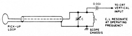
Fig. 5. Coupling rf to oscilloscope.
If the power level of the transmitter and the deflection sensitivity of the CRT are well matched, sometimes merely a simple tee fitting can be inserted in the transmission line. The signal available at the arm of the tee can be applied directly to the vertical input to the oscilloscope through a blocking capacitor. At high power levels, the center conductor of the stem of the tee can be removed and replaced by a short stub which couples capacitively to the center conductor that remains in the cross arm of the tee. Modified tees of this sort can be constructed with different coupling coefficients for different power levels.
Transmitter Testing
With the oscilloscope coupled to the transmitter, the two-tone signal can now be injected into the transmitter through the mike jack. Set the transmitter's mike-gain control to its normal position for SSB operation, and make any required adjustments in input signal level to the transmitter with R9, the output-level control of the main circuitry. S2 can be momentarily set for continuous output while adjusting R9. On rigs with an ALC indicator, adjust R9 so that ALC activity just starts to occur; otherwise set R9 by whatever method is usually used to adjust the mike gain.
Be sure to use a dummy load out of courtesy to other amateurs. After setting R9, don't forget to return S2 to tne pulse position.
With the two-tone signal being fed to the transmitter and the output dissipated in the dummy load, the envelope of the test pattern should be observed on the oscilloscope. Photo D is an example of what the display should look like. Examples of what the pattern should not look like can be found in the references as can be additional examples of correct two-tone envelope patterns.(4)(6)(7)(8) If any deviation from the correct pattern can be seen by the naked eye, hen the actual level of spurious products has already reached moderate levels.
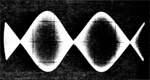
Photo D. Correct two-tone test pattern as displayed by the monitor scope. Coupling was by use of a tee in the transmission line.
In other words, by the time the human eye can notice distortion in the two-tone test envelope pattern, actual spurious output products as would be shown by a spectrum analyzer (IMD products as well as insufficient carrier suppression) have already reached an inacceptably high level of -25 to -20 dB down from the PEP output level.(4) Needess to say, if you can see any distortion in the two-tone pattern, adjustment of the transmitter and/or amplifier is necessary. Hopefully, you will be able to obtain the correct pattern of Photo D.
Input Power Measurement
If S2 is momentarily set or continuous application of the two-tone test signal and the indicated dc input current is observed, the PEP input current being drawn can be calculated by I(PEP) = 1.571 x I(dc) - 0.570 x 1(0), where I(PEP) is the PEP input current, I(dc) is the dc input current indicated by the meter, and I(0) is the resting current drawn by the final with no output sigial. Apply the continuous two-tone signal only long enough to obtain the readng, otherwise you might overheat the final amplifier. Also, measure the supply voltage to the final while the continuous two-tone signal is applied. This is necessary because most supply voltages drop significantly under loaded conditions. The product of the loaded supply voltage and the PEP input current then give the PEP input power to the final amplifier under test.
Output Power Measurement
Besides checking for distortion, the oscilloscope is a useful instrument for measuring peak instantaneous output power. Remember that peak instantaneous output power is not PEP output power. PEP output power is the rms power of one complete rf cycle occurring during periods of peak modulation when transmitting SSB or under key-down conditions during CW operation. Note-that as with other methods of measuring rf power, the transmission line must be properly terminated if accurate measurements are to be obtained.
If a convenient display that fills between 40% to 90% of the screen can be obtained with the direct-connection technique using a normal tee fitting in the transmission line, it is necessary only to calibrate the vertical deflection of the oscilloscope directly in volts per graticule division. PEP output power is then given by: P = E2/(2Z), where E is the peak instantaneous voltage as measured by the oscilloscope (1/2 of the total pattern height) and Z is the characteristic impedance of the transmission line. Calibration of the vertical-deflection factor can easily be obtained by applying 60 Hz ac to the vertical plates from an appropriate transformer. Be sure to measure the voltage with an ac voltmeter; don't rely on the rated voltage of the transformer. Remember that the voltmeter will almost certainly read the rms voltage, not the peak-to-peak voltage which is what the oscilloscope will display.
If one of the other indirect coupling methods is used, then there will be an arbitrary but constant factor relating graticule divisions to the peak-to-peak rf voltage displayed. One method of determining this calibration constant is to insert a calibrated rf wattmeter into the transmission line and measure the rf power delivered by the transmitter when set for normal CW operation. At the same time, note the height of the pattern on the oscilloscope screen. If the wattmeter reads average or rms power, then the peak instantaneous rf voltage is given by: E = √(2×P×Z).
Alternatively, an rf ammeter can be inserted into the transmission line to measure the rms current, and then the peak instantaneous rf voltage is given by: E = 1.414×I×Z. Remember that these values must be multiplied by two to obtain the peak-to-peak value which represents the full pattern height.
Another method of determining the calibration constant is to measure the rf voltage developed across a dummy load with an rf voltmeter probe connected to a VTVM or other high-input impedance voltmeter; these rf probes usually are set up to measure rms voltage, and this value must be multiplied by 2.828 to obtain the peak-to-peak value.
Conclusion
Once the monitor scope is working properly and, if desired, it has been calibrated for output power, it can be left in the transmission line as a permanent indicator of correct station operation. The pulsed two-tone pattern can be used briefly to tune up the rig for maximum power without distortion, and during speech transmission, the voice-pattern peaks can be examined to be sure they are not exceeding this level. In this manner, peace of mind for the doubting Thomas can at last be obtained.
References
- Goodman, Byron, W1DX, "Linear Amplifiers and Power Ratings," QST, August, 1957.
- Lange, Walter, W1YDS, "A Pulsed Two-Tone Test Oscillator," QST, September, 1965.
- Graeme, Tobey, and Huelsman, Operational Amplifiers, Design and Applications, McGraw-Hill, New York, 1971.
- Radio Amateur's Handbook, Chapter 12, ARRL, Newington CT, 57th Edition, 1980.
- Amidon Associates, 12033 Otsego St., North Hollywood CA 91607.
- Ehrlic, Robert W., W0JSM, "How to Adjust Phasing-Type SSB Exciters," QST, November, 1956.
- Ehrlic, Robert W., W0JSM, "How to Test and Align a Linear Amplifier," QST, May, 1952.
- Blakeslee, Douglas, W1KLK, "Testing a Sideband Transmitter," QST, September, 1965.