Underwater radio communication
How far can we communicate underwater in the sea or in a lake? How large is the signal attenuation and what frequency can be used? Could we use 1.8 MHz?
In the following paragraphs, we attempt to answer some of these questions.
One could ask why a radio amateur enthusiast might be interested in underwater communications. Well, he could be interested in skin-diving and wish to set up a communications link with the surface, or perhaps he might be interested in radio controlled boats and wish to try his hand at model submarines! On the other hand, he might just be interested in another area of experimentation because here is a field, relatively untouched by the amateur fraternity, involving different transmission techniques, different antenna designs and different equipment environmental problems.
The scope of this article concerns the transmission characteristics of radio waves underwater and the extent to which the radio amateur might make use of these characteristics.
Water conductivity
Water in its pure form is an insulator, but as found in its natural state, it contains dissolved salts and other matter which makes it a partial conductor. The higher its conductivity, the greater the the attenuation of radio signals which pass through it.
Conductivity (σ) varies with both salinity and mperature. Sea water has a high salt content and high conductivity varying from 2 mhos per metre in the cold arctic region to 8 mhos per metre in the warm and highly saline Red Sea. Average conductivity of the sea is normally considered to be about 4 mhos per metre. What this means is that one metre cube of sea water has a conductivity of 4 mhos or a resistance of 0.25 ohm, it reciprocal.
So called fresh water has lower conductivity and as a guide to this, a sample analysis of Adelaide water taken in 1983 has been used. This sample was taken from an area principally supplied by the Barossa reservoir and the analysis shows total dissolved salts as approximately 300 mg/litre and a conductivity of 0.0546 mhos per metre. How close this is to the average waters in lakes anr rivers in Australia is not known, but as it at the only water on hand, it has been used as a reference.
Attenuation
Attenuation of radio waves in water (and, in act, in any conducting medium) increases both with increase in conductivity and increase in frequency. It can be calculated from the follow formula:
Attenuation (a) in dB/metre ![]()
where f - frequency in hertz σ - conductivity in mhos/metre
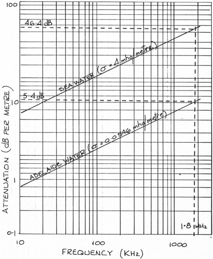
Figure 1: Underwater Attenuation versus Frequency.
Figure 1 illustrates attenuation as a function of frequency for sea water and Adelaide water. Attenuation in sea water is very high and to communicate at any depth at all, it is necessary to use very low frequencies (10 to 30 kHz) where attenuation is in the order of 3.5 to 5 dB per metre. Operation in the lowest frequency amateur band (1.8 MHz) is out of the question at 46 dB per metre.
The potential for operation in fresh water is much better. Using the Adelaide water sample, attenuation at 10 kHz is only 0.4 dB per metre rising to 5.4 dB per metre at 1.8 MHz.
Refraction or interface loss at the surface
When EM waves travel from air to water or water to air, there is a refraction loss due to the change in the medium. This loss can be calculated from the following formula:
Refraction loss (dB) = 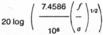
In sea water, this loss is quite high and in the vicinity of 60 dB for the low frequencies normally used. If communication is required from surface to underwater, path loss can be reduced by connecting the surface equipment to an antenna under the surface so that the refraction loss is eliminated.
Figure 2 illustrates refraction loss as a function of frequency for sea water and Adelaide water. It can be seen that refraction loss falls with an increase in frequency and in the case of the fresh water, this loss is down to 27 dB at 1.8 MHz which is quite attractive from an amateur radio point of view.
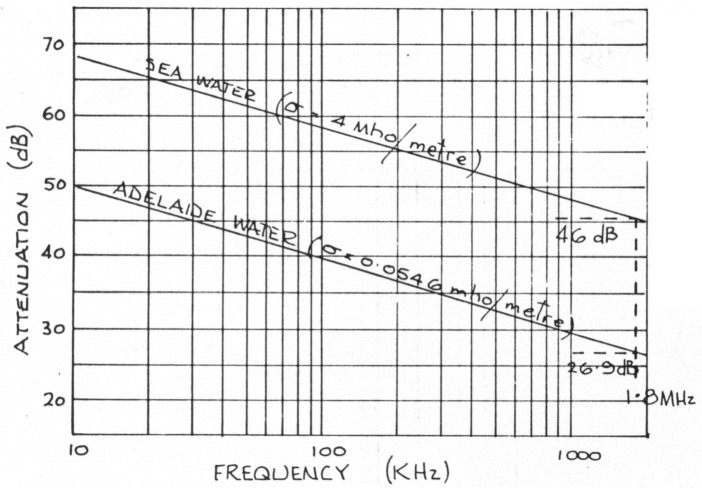
Figure 2: Air to Water Retraction Loss as a Function of Frequency.
Wavelength in water
The wavelength in water is but a fraction of that in space and is calculated from the following formula:
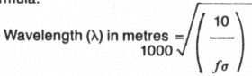
Figure 3 plots wavelength versus frequency. In sea water, wavelength at 10 kHz is only 15.8 metres compared to 30 km in space. In fresh water the reduction in wavelength is not so dramatic but still quite considerable. At 1.8 MHz, wavelength is 10.1 metres compared to 167 metres in space. This reduction is wavelength leads to some considerable differences in antenna engineering with an underwater dipole at 1.8 MHz being only a few metres long.
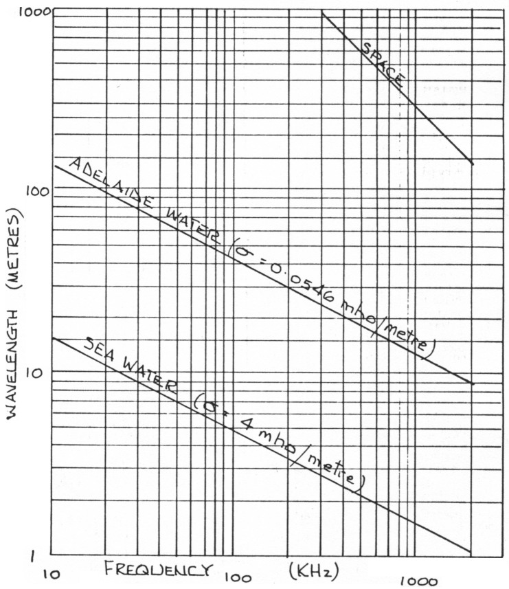
Figure 3: Wavelength versus Frequency.
Transmission options
The lower the frequency, the lower the attenuation in water and the better the potential for communications. Unless a band of frequencies could be approved for amateur use in the VLF region, the options for amateur radio are restricted to 1.8 MHz and communication in fresh water. A few transmission examples for this application will be discussed and these will be based on the following assumptions:
- Radiated power is 0 dBW (referred to one watt developed in a half wave dipole). All other measurements are in decibels referred to that level.
- Receiver bandwidth = 3 kHz.
- Minimum discernible receive level at receive antenna = 10 dB above thermal noise (KTB) ie -153 dBW (for 3 kHz bandwidth).
- Atmospheric noise at 1.8 MHz = 35 dB above KTB (taken from published noise charts) ie -128 dBW for 3 kHz bandwidth.
- Attenuation in fresh water = 5.4 dB/metre (from Figure 1 at 1.8 MHz).
- Water/air refraction loss = 27 dB (from Figure 2).
Figure 4 shows the receiver submerged and the transmitter above the surface. The signal path is subject to 27 dB air/water interface loss. Atmospheric noise is also attenuated by the interface and path loss and minimum receive level is set by the sensitivity of the receive system (not affected by atmospheric noise). Maximum length of the water transmission path works out to 23 metres.
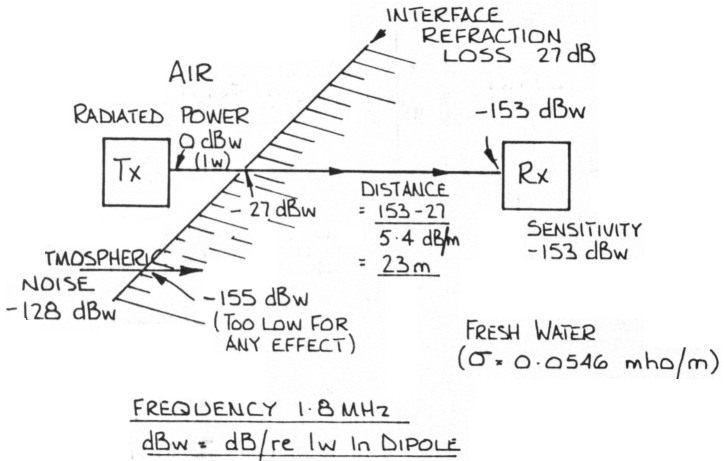
Figure 5 reverses transmission direction so that the transmitter Is submerged and the receiver is above the surface. In this case the minimum receive level is set by the atmospheric noise (well above the receive system sensitivity). Because of this, the maximum length of water transmission path is reduced to 18.7 metres.
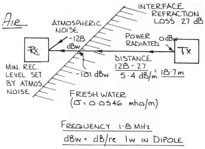
Figure 5: Transmission Path Fresh Water to
Figure 6 submerges both transmitter and receiver, eliminating the air to water interface loss of 27 dB. This extends the maximum length of water transmission path to 28 metres.
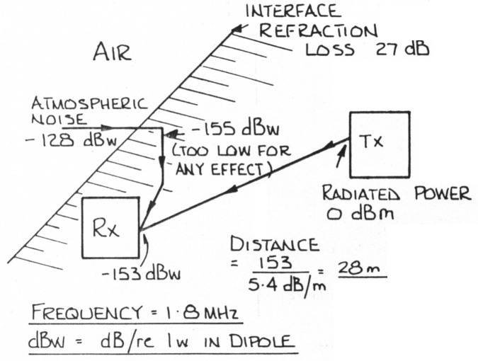
Figure 6: Transmission Path - Fresh Water Transmitter and Receiver Both Submerged.
We now turn our attention to transmission in space. Beyond one wavelength from the transmitting antenna, field strength in space varies inversely with distance; ie the signal is attenuated 6 dB each time the distance is doubled and attenuation from a point one wavelength from the antenna to a distance d is equal to 20 log (d/λ).
Referring now to Figure 7, we have a transmitter with a reference power 0 dBW at wavelength and this point is 1000 metres (or six wavelengths) from the water surface. Power level at the air/water interface is -20 log 6 = -15.6 dBW and transmission for a further 20 metres underwater is still possible.
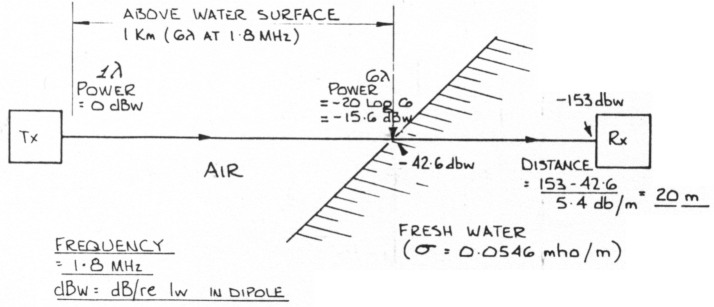
Figure 7: Transmission Over a Large Distance Above the Surface to a Submerged Receiver.
Taking this type of transmission a little further, we now examine Figure 8. Here we have both transmitter and receiver below the water surface but 1000 metres apart. Communication over this distance via the water is impossible but the signal can leave the water near the transmitter, travel via the air path and re-enter the water near the receiver. The signal suffers the interface loss twice (ie 3 dB) but attenuation over the 1000 metres is limited to that of the air path. So here is another technique by which two underwater stations might communicate over quite a large distance, limited essentially by the depth in water at which the stations are based.
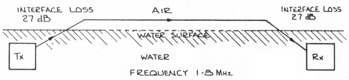
Figure 8: Communication Between Two Submerged Stations vla Air Path.
In the examples given, actual transmission distance underwater is limited from 18 to 30 metres. This distance can be increased by increasing power or decreasing frequency. Increasing the radiated power to 100 watts would give 20 dB gain or an extra underwater distance of 3.7 metres (not a large increase). If a frequency of 100 kHz were available, attenuation would be 1.28 dB/metre and taking the example of Figure 6, distance would recalculate to the greater value of 120 metres. At this frequency, however, interface loss increases to 40 dB and in the example of Figure 4 (which includes interface loss) the distance would be a lesser 88 metres, but still greater than for 1.8 MHz.
Another point to consider, is that Adelaide water is not renowned for its purity of dissolved (or undissolved) matter and it is possible that water in lakes and rivers elsewhere might have lower conductivity than that of the Adelaide sample.
Antennas
Design of underwater antennas is beyond the scope of this article, but a few interesting details can be discussed. Published references indicate that loop antennas, long wires and dipoles have been successfully used underwater at very low frequencies, their physical dimensions, in terms of a space wavelength, being much less than their equivalent in space.
Antenna conductors are insulated from the water to prevent leakage current direct to the conducting medium, but there is still coupled conduction into the medium which causes the radiation resistance to be considerably lower than that of the equivalent antenna in space. A radiation resistance of a few ohms can be expected for a half wave dipole.
There is also the question of polarisation and directivity. According to Moore(2), a submerged horizontal electric dipole is equivalent in its field to a weaker vertical antenna at the surface. Most of the energy, radiated upwards from the antenna, is refracted at the surface into a vertically polarised, almost horizontally travelling wave, above the surface. This phenomenon helps to explain the technique used in Figure 8 to transmit signals horizontally above the water surface and to receive them in the reverse process.
Moore also points out that attenuation between one side of the submerged antenna and the other, is so great that a major contribution to the field at any point is primarily due to the nearest point on the antenna. Thus coordinates on an antenna pattern in a conducting medium are meaningless. There is, of course, a null off the end of a dipole and hence horizontal dipoles are more satisfactory than vertical dipoles for communication via the surface.
Antennas used in the sea have made use of the conducting sea as the actual radiating element. The signal is either coupled to the sea via connecting electrodes or by inductive coupling from an insulated loop.
These techniques are possibly impractical for fresh water with much lower conductivity.
Sea water
As discussed earlier, attenuation of radio signals in sea water is so great that communication further than just below the surface is not possible unless very low frequencies (10 to 30 kHz) are used. Even if permission could be obtained to use frequencies in this band, there are other difficulties facing the amateur enthusiast:
- Air to water refraction loss in this band is in the order of 60 to 70 dB.
- Massive antenna dimensions are required, particularly for the above the surface antenna. (Even at 30 kHz, a wavelength is 10 km). Large transmitter powers are usually required to compensate for the high antenna losses inherent in the shortened low frequency antenna.
- Atmospheric noise peaks to about 160 dB above thermal noise (KTB) at 10 kHz, limiting the minimum discernible receive level.
Other conducting mediums
Whilst the discussion has concentrated on transmission through water, the theories outlined can equally be applied to other conducting mediums such as the earth's crust. Typical applications include radio communications in underground shafts and caves.
The conductivity of the earth's crust varies widely with conductive over- burden between 10-4 and nearly 1 mho per metre and low conductivity rock less than 10-5 ohms per metre. Quite clearly, the success of the underground communications depends on the geo. logical make up of the surrounding terrain.
Conclusions
Radio communication under the sea is not an attractive option for experiment by the radio amateur as it requires the use of very low frequencies, large antenna systems and very high powers.
Fresh water lakes and rivers have much lower electrical conductivity than the sea and underwater transmission distances (or depths) up to 30 metres appear feasible using the lowest frequency amateur band of 1.8 MHz. Even larger distances (or depths) could be achieved if a lower frequency band allocation were made available.
Communication between underwater stations or between a surface station and an underwater station could be achieved over much larger distances by utilising a transmission path above the surface and tolerating the air to water refraction loss.
Similar communications could be carried out from underground depending on the conductivity of the surrounding over-burden or rock.
References
- Reference data for radio engineers, ITT Chapter 27. Radio noise and interference.
- Moore, Richard R. Radio Communications in the Sea, IEE Spectrum, Vol 4, Nov 1967, pp 42-51.
- Hansen, R C. Radiation and Reception with Buried and Submerged Antennas, IEEE Transactions on Antennas and Propagation, May 1963.
- Watt, Leydorf and Smith. Notes regarding possible field strength versus distance in earth crust wave guides.
Symbols used in text
| σ (Sigma) | Electrical conductivity (mhos/metre). |
| f | Frequency (Hertz). |
| λ (Lambda) | Wavelength (metres). |
| dB | Decibels. |
| dBW | Decibels reference one watt. |
| α (Alpha) | Attenuation constant (dB/metre). |
| d | Distance (metres). |
VK5BR, Lloyd Butler.