A frequency and level standard
A little black box and some digital pulse magic produce a frequency-stable, high-level generator
A good RF signal generator needs an effective electrical shield around its generating circuit. Without such a shield, it would not be possible to guarantee an accurately determined output level over a wide range of frequencies. In other words, the output attenuator would lose its credibility.
Shielding an RF circuit requires more than just placing the components behind a metal wall. Leakage and radiation will occur from almost anything electrical that happens to protrude from the circuit enclosure. Sometimes a rather sophisticated filter system is required for stopping the interference that would otherwise spoil the output-level calibration, particularly at low levels and at high frequencies.
This shielding requirement is only one reason a good RF signal generator is usually an expensive piece of test equipment, and difficult to build yourself. For me, it was the reason behind the rather unusual design of the frequency and level standard, which, of course, is just another name for a signal generator.
Design concept
In principle, the idea is simple. A circuit contained in a hermetically sealed box can't have any filter problems if there's nothing to filter in the first place. That's why I thought of designing a signal source without external controls, power cable, tuning, or level meter - just a box with an output connector. Everything except the output is kept inside.
Thinking a bit further, putting such a drastic principle into practice was not as easy as it sounds, and a few concessions were unavoidable here and there. For example, it's difficult to tune an oscillator and to have its frequency displayed through a solid shield. Consequently, I had to restrict the output signal to cover only a certain number of predetermined frequencies.
The simplest way to obtain many fixed frequencies simultaneously is by adopting the frequency-marker principle; that is, by deriving harmonics from a crystal oscillator. This also guarantees good frequency stability,. To keep the many signals separate from each other they must be labelled; I gave them, therefore, different amplitudes, making them clearly distinguishable. This was done with the help of a very elementary digital processing circuit.
A simple action - such as flipping a switch - could pose a problem if it had to be done through a metal shield. But this is also no problem: mercury switches mounted inside the circuit can be actuated simply by turning the box to a different position.
The part that needs most switching, the variable output attenuator, is kept outside the shielded enclosure. This allows the signal generator to produce a uniform, but accurate, signal level over a wide frequency range. In fact, it turns out that it's not only the generator itself, but also the variable attenuator that determines the eventual level accuracy at higher frequencies. And the outboard attenuator can be easily replaced by an improved version at a later date.
The cost of the active components (six ICs, including the voltage regulator) should come to not much more than $3.00. To sum it up, at least for many applications, the box-with-plug idea works the way I hoped it would: as a good signal generator that is neither expensive nor difficult to build.
Synthesizer
Many people who've tried to calibrate a receiver frequency scale using a frequency marker have had the experience of being confused by the different, but look-alike, signals. It is therefore an advantage to introduce signals that belong to a different order in the spectrum hierarchy. First the 1-MHz markers, for instance, then the 100-kHz markers, and so on. Usually this is done by turning a switch.
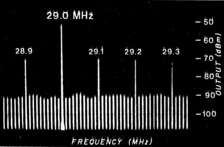
Fig. 1. Typical output display spectrum as seen on a frequency-spectrum analyzer. Multiples of 100 kHz harmonics have signal strengths corresponding to the standard S9. The MHz markers are about 20 dB stronger; the 10-kHz markers are 20 dB weaker.
To avoid using such a switch, I tried a different method. The coarse markers were labelled by emphasizing their amplitudes (fig. 1). After frequency division of a 1-MHz crystal-oscillator signal, pulses of different lengths arrive at the NAND gates. The product is used to interrupt the stream of 1-MHz oscillator-output pulses at regular intervals by longer or shorter spaces (fig. 2).
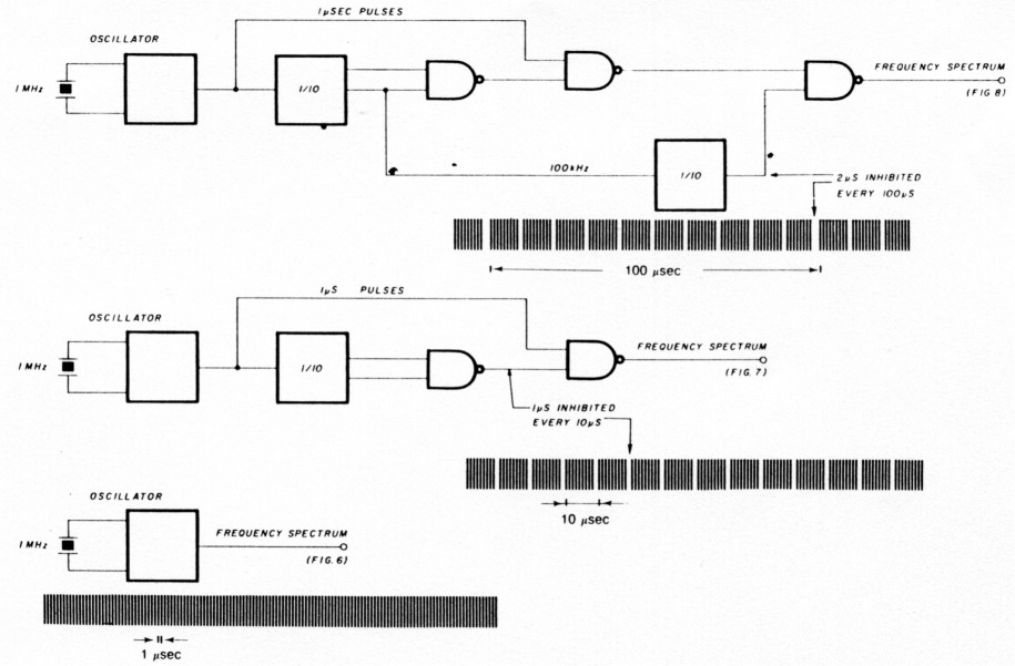
Fig. 2. Method by which the frequency spectrum is synthesized by creating patterns in a digital pulse sequence.
The underlying mechanism that produces the different phenomena may be easier to understand when you realize what the pulse sequence would look like if the polarity had been reversed. Tuned circuits in a receiver recognize certain patterns in the stream passing by and therefore respond to certain rhythms. Thus, for example, the one-pulse space in the otherwise steady flow of 1-µs (1-MHz) pulses represents, in fact, a pulse of relatively longer duration. If such an event occurs regularly every 10 µs, it is capable of causing a response in a circuit tuned to a multiple of 100 kHz (being the repetition rate of the space).
The reason amplitudes of the 1-MHz markers stand out from the rest is not difficult to see. The train of 1-µs pulses with each 10th pulse removed produces more energy in a circuit tuned to a 1-MHz multiple than to one tuned to a 0.1-MHz multiple (where, at the same time, the circuit has to manage with only one out of ten pulses).
The two-pulse spaces responsible for the 10-kHz markers (occurring every 100 µs) produce energy that must be shared over 100 times as many signals in the frequency spectrum. This explains why the 10-kHz markers are so much weaker than the others. Of course, all this tampering with pulses makes the total architecture rather complex. It is, therefore, not surprising to find that there's a practical limit to where the results remain acceptable, and where further refinements would create a less orderly spectrum. What happens is that if the mixture of pulses and spaces in between gets too complex, less-warned patterns become recognizable. This results in poorly determined amplitudes. Therefore only the 100 kHz position (only multiples, all with identical amplitudes) should be used as a level standard. The spectrum-analyzer pictures show how the amplitudes tend to become irregular as the frequency spectrum becomes more complex.
Thus the imperfection is not so much the result of what a typical analog thinker (as many Radio Amateurs appear to be) might suspect: the wiring. Digital circuits are remarkably tolerant of construction-related problems such as breakthrough or crosstalk - and, for that matter, of poor layout, messy wiring, and horrible-looking breadboard creations. What is also appreciable is that from .the synthesizer output onward, only the absolute amplitude may change. The amplitude ratios between the different orders of frequency, once they have been encoded into a digital pattern, are not likely to be changed by following wave-shapers, amplifiers, or other analog circuits.
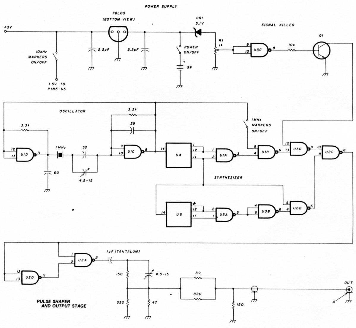
Fig. 3. Schematic diagram. The entire circuit, battery included, is contained in a closed metal box which is electrically connected to the circuit ground only through the coaxial cable to the output connector at point A. U1 and U3 7400; U2 74S00; U4 and U5 74SL90.
Figure 3 shows the circuit as it was eventually adopted; fig. 4 shows the socket connections of the ICs. Note that an electrolytic capacitor is provided at each individual IC for additional voltage protection.
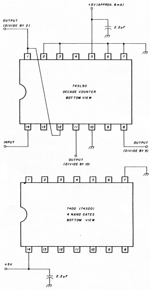
Fig. 4. Socket connections of integrated circuits used in fig. 3.
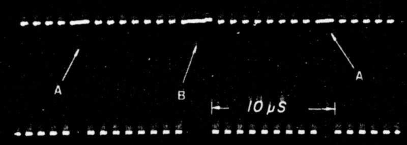
Fig. 5. Synthesizer output signal as displayed on oscilloscope. At A one pulse is inhibited, repetition rate 10 µs. At B two successive pulses are inhibited, repetition rate 100 µs.
Figure 5 shows an oscilloscope display of a detail from the synthesizer output pattern showing some 1-pulse spaces (indicated by A) responsible for the 100-kHz signals, as well as the 2-pulse spacing (B) that produces the 10-kHz markers. Figures 6, 7, and 8 show the different frequency spectra that are created by the pulse patterns given in fig. 2.
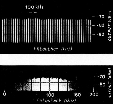
Fig. 6. 100 kHz position. Top: typical segment of output frequency spectrum as displayed on spectrum analyzer. Each signal frequency is a multiple of 100 kHz and has a level of -73 dBm ± 1.5 dB, up to at least 30 MHz. Bottom: spectrum displayed over full usable frequency range. Although signals are no longer individually distinguishable, the display shows signal levels within ±2 dB up to 160 MHz.
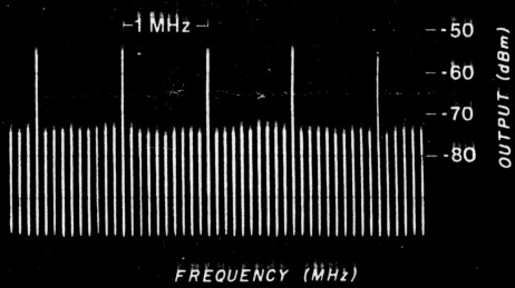
Fig. 7. Position: 1 MHz + 100 kHz. Spectrum of 100-kHz marker signals, with 1-MHz marker amplitudes emphasized by approximately 20 dB.
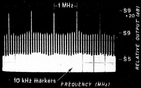
Fig. 8. Position: 1 MHz + 100 kHz + 10 kHz. Spectrum is shown with all markers in operation.
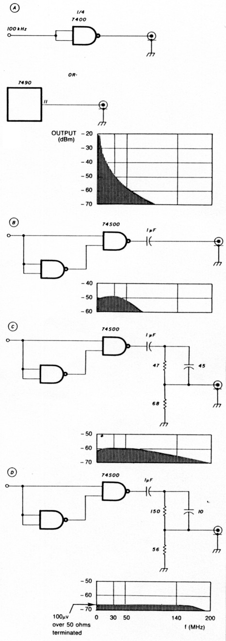
Fig. 9. Examples of output-stage configurations and the effect on the frequency response. In all cases the output is terminated in 50 ohms.
Output stage
The output stage consists mainly of a pulse shaper, or "harmonic producer," based on the fact that the shorter the pulse duration, the more frequencies are produced, and consequently the frequency spectrum will be wider and the harmonic amplitudes more uniform, though lower.
How short should the pulse duration be for obtaining a reasonable compromise between frequency range and output level? For lack of more specific information in the otherwise plentiful literature on frequency markers, I investigated a few circuits I found in Amateur Radio publications.
The output of a 7400-type NAND gate turns out to have an impedance of about a few hundred ohms and could, if necessary, be safely connected to a 50-ohm load. (The IC would even survive a full DC short from its output terminal to ground, if it ever came to that.) However, to permit a proper match into a 50-ohm device, such as an attenuator, a small network is inserted. This also permits an increase in frequency response at the high-frequency end of the spectrum.
Figure 9 illustrates some of the networks that I tried. Note the important improvement by the one shot in fig. 9B. This simple circuit turns out very short pulses indeed. In this circuit, the last NAND gate receives the pulse directly at its top input. The pulse is inverted at the bottom input, and is delayed only by another NAND which acts as the inverter. As the output of a NAND gate is low only if both inputs are high, the total effect could perhaps be compared with letting a signal rush through the circuit, and immediately slam the gate shut behind it, chopping its tail. Thus, using an ordinary 7400, all output pulses have a duration that can't be longer than about 10 nanoseconds, the delay time of the inverter. The circuit produces adequately short pulses for creating a reasonably flat frequency response that covers all HF bands, requiring only a slight correction.
The 7400 also exists in a more than three-times-asfast Schottky version, the 74S00. This device produces even shorter pulses and makes it possible, at least with some correction again, to create a flat response that comfortably includes the 2-meter band. At the time the spectrum (which starts to roll off at 160 MHz) reaches 400 MHz, the amplitudes have dropped by about 15 dB. This would still make a good frequency marker for the 70-cm band.
In the final circuit (fig. 3) an extra 50-ohm, 6-dB attenuator is inserted. This puts the output level at -73 dBm and provides isolation between the frequency-correcting network and a possible capacitive load at the output connector.
The -73 dBm level was chosen for a good reason. It allows sufficient compensation of the frequency response for including the 2-meter band. It also corresponds with the IARU-recommended S9 level at HF bands. By leaving the output unterminated, the open-circuit output voltage produced by every multiple of 100 kHz (100 kHz position) is 100 µV, or S9 at the high-impedance input terminal of an HF receiver. Terminated into a 50-ohm receiver antenna input, the voltage drops to the IARU-recommended 50 µV.
Once the receiver S-meter has been calibrated for this level, the other S-points are easy Po determine by halving the voltage for each lower S-point on tae scale. To put it more practically, each S-point change in level corresponds to 6 dB. Just a few examples: S8 = -79 dBm, S3 = -109 dBm.
Somewhere in the last NAND lies the borderline between the digital and analog sections of the circuit. From this point onward, carefree wiring concepts are better abandoned. The resistor network between the NAND and output connector requires careful layout consistent with good VHF practice. The resistors are best mounted free from each other and from other components, and with their wires as short as possible. Printed-circuit technique is not recommended here.
The shield box is electrically insulated from the circuit ground except at the output connector, through the coaxial cable.
Oscillator
Experimenting with ICs of the 7400 series, one may find that the different blocks, with their low input and output impedances, aren't the ideal elements for building a crystal oscillator. If the crystal isn't very active, the oscillator won't work. Nevertheless, the reason for using this circuit is that the NANDs - four of them combined in one IC - happened to be available, and they draw supply current whether they are used or not.
If the circuit doesn't work, it may well be possible to wake up a lethargic crystal by using different values for the resistors and capacitors in the oscillator circuit. However, it's also possible to overdo it, causing the oscillator to produce parasitics. In case of persistent recalcitrance, any other oscillator using one or two discrete transistors may do the job just as well, consuming only a few milliamperes of extra current.
Power supply
One disadvantage of the closed-box technique may be that it doesn't leave much opportunity for monitoring the battery-supply voltage. That's why a voltage regulator, supplied by a battery that has some voltage to spare, is incorporated. The 9-volt battery can be drained to the point at which its actual voltage drops to 6.4 volts before the regulator gets in trouble trying to keep up its 5-volt output (that is to say, this is what I found; the 78L05 specifications state a minimum input voltage of 7 volts). As soon as the regulator output becomes affected, the RF output level of the total circuit becomes unreliable. Responsibility for this is mainly the last NAND in the output stage, producing pulses with lower amplitude and consequently less energy.
The problem of the aging battery is solved by applying a form of euthanasia. The "signal killer" circuit is based on the principle that it is better t0 have no signal at all than one on which you cannot rely. As soon as the battery drops below 6.4 volts, the RF output signal is cut off abruptly (fig. 10), before it can cause incorrect test results. This is done by blocking a NAND in the main signal path through a NAND inverter and a transistor.
When the appropriate moment arrives, the act is performed swiftly, even in case of a very slowly deteriorating battery voltage. The threshold is set by potentiometer R1 (fig. 3) to make the RF output signal disappear just before a reduction in amplitude occurs.
Because an output signal that suddenly disappears can be disconcerting, I found it useful to provide a means of alerting the user to the imminent demise of the battery. If the box fails to deliver its output signal, just turn it to the position 1 MHz + 100 kHz + 10 kHz. If only the 10-kHz markers are still present, this is a sign that the malfunction of the generator is the result of too-low battery voltage, and that there's no reason to expect anything worse than having to replace the battery.
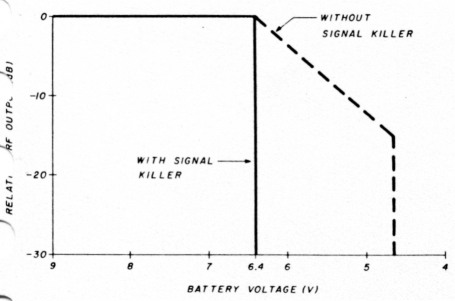
Fig. 10. RF output as a function of battery voltage. An unnoticed drop in RF output level, resulting from an exhausted battery, is made impossible by the action of "signal killer."
The battery is normally switched on and off by a mercury switch, a miniature glass bulb in which a droplet of mercury makes contact between two wires, appending on the position of the device. With some three-dimensional imagination, it's not difficult to see how, using a switch, a circuit can stay switched on in a maximum of three different positions of the box. This is done by mounting the switch in the circuit wiring at an oblique angle with respect to the three axes of the box. Similar switches are used for switching the 1-MHz and 10-kHz markers.
If mercury switches are difficult to obtain, it shouldn't be difficult to think of something else, such as one or more reed switches and a movable magnet, for example. Another method would be to use a steelball (a ball bearing, for example) that can roll around inside a little plastic box with contact wires, or in a little box made of printed-circuit board (fig. 11).
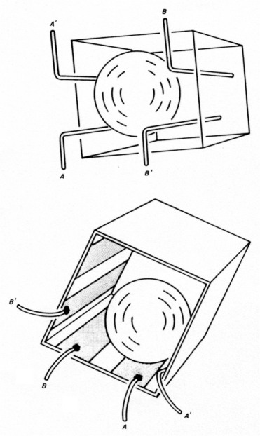
Fig. 11. Substitutes for a mercury switch showing suggestions for an inclination switch using a steel ball. In position sketched: a-a' closed contact, b-b' open contact.
The total battery consumption at 9 volts is about 43 mA with all markers operational, or about 36 mA in the 100 kHz position.
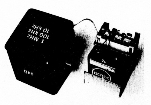
The frequency and level standard outside its enclosure. Normally the entire circuit, power supply, and all control elements are inside the black metal box; thus all RF leakage is eliminated without the need for any filtering.
Attenuator
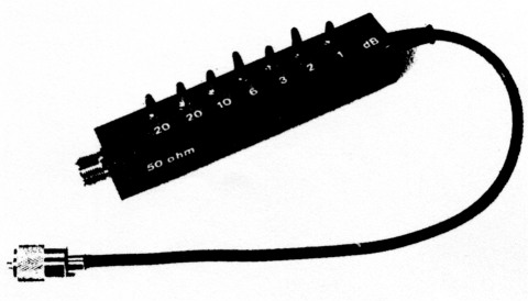
The type of outboard step attenuator shown in the fotograph has been described already in many Amateur publications. In this case, miniature toggle switches and 1/4-watt carbon resistors are used. The resistors are mounted on the solder lugs of the switches, with their leads kept as short as possible. For the rest of the wiring, copper braid (taken from the coaxial cable) is used, soldered over the full length of the solder lugs. Braid is not essential insofar that it doesn't seem to extend the flat portion of the frequency response; however, I found that it can give a considerably smoother result at VHF.
Production tolerances in the resistor-manufacturing industry appear to have greatly improved over the last decade. At one time, a 10-percent resistor was almost bound to show a tolerance between 5 and 10 percent.
Today it's not unusual to find that ordinary 10-percent resistors are in fact not much more than 2 percent off the mark. And as more accurate ohmmeters become available to Radio Amateurs, it's no longer difficult to obtain reasonably precise resistors.
The required values for the attenuator are obtained by parallel combinations. In each combination it is mainly the lower-value resistor that is critical and which should preferably be within 1 to 2 percent. (Tolerances of resistors are like those of voltages, and the same rule-of-thumb applies: for small variations, each percent corresponds to 0.1 dB.) Alternatively, each combination should be brought as close as possible to the ideal value by selection and trial and error, using an accurate (digital) ohmmeter (fig. 12).
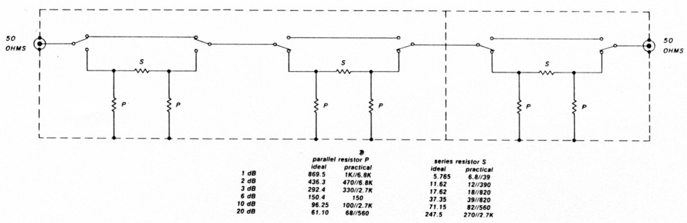
Fig. 12. Design parameters of toggle-switch attenuator with standard-value resistors. Practical column lists parallel combinations that most nearly meet ideal values. (All values in ohms.) Note: // means placing the two resistors in parallel.
Most descriptions of this type of step attenuator remain rather vague about the performance, particularly at higher frequencies. Therefore, fig. 13 may be of interest, because it shows the test results of this home made attenuator, built with no particular care other than ordinary construction techniques. The device is accurate within 1/10 of a dB or thereabouts, up to 65 MHz; that is, as accurate as the resistors could be selected with the available DC ohmmeter.
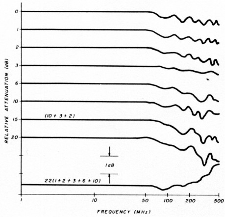
Fig. 13. Test results of home made attenuator. Frequency response is shown at each setting, as well as at some combinations. Note absence of any appreciable discrepancies up to 65 MHz.
Figure 13 also shows the reason for the apparent reluctance to publish test results: at VHF precision tends to become questionable. Nevertheless, the general performance is still within the tolerance of the signal generator, about ± 1 dB uncertainty at 144 MHz.
That the discrepancies are mainly the result of the many twists and turns in the signal path through the switches is also clearly demonstrated. Even with all attenuators in the OUT position (0 dB), the wavy character of the curve remains. This gives hope; it's not impossible that (cheaper) slide switches and N-type coaxial connectors would make an improvement on VHF.
Calibration
The accuracy of the frequency can be checked and corrected by adjusting the oscillator trimmer while comparing a signal with one of the short-wave standard signals such as WWV in the USA, or GDF in Europe. Because the circuit doesn't contain any variables in the form of tuned circuits, the output level of -73 dBm should be fairly easily reproducible for HF by using the components as described. Up to, say 30 or 40 MHz, the frequency response should remain flat within reasonable limits, even if the output trimmer is simply replaced by a 10 pF fixed capacitor.
In the multitude of standard-size 100-kHz harmonics there appear to be two exceptions where the amplitude seems to behave a bit freakishly: at 100 kHz itself and at 1MHz. I found relative levels of -4 dB and -10 dB, respectively. As yet I have no fully satisfactory explanation to offer for the phenomenon; it's difficult to speculate to what extent these findings may be typical for the circuit.
The output can be calibrated by comparing the level of one of the 100-kHz harmonics (except at 100 kHz and at 1 MHz) with that of a signal from an RF generator with a reliable output attenuator, using a radio receiver as a frequency-selective balance detector. A signal-strength meter is not absolutely essential. By comparing two beat tones, one immediately after the other, providing that they both have the same pitch, one should be able to match levels well within 1 dB.
However, a professional RF signal generator could be difficult to procure, and for the average Radio Amateur a more common audio generator might be more easily available. Audio levels are more accurately determined using an audio voltmeter or an oscilloscope. Most audio generators cover 200 kHz, and a level comparison could be made on a long-wave radio receiver, using an audio meter or the human ear. After all, the 200-kHz harmonic is just as strong as any other harmonic in the entire HF spectrum of the generator and, even if it sits at an extreme end of the range, it provides a perfectly typical specimen upon which to base the level calibration.
In case level corrections appear to be necessary, the resistors in the attenuator between output trimmer and coaxial cable can be replaced to change the 6-dB attenuation into a different value. Figure 13 supplies the data.
PA0CX, Hans Evers.