Near linear tuning with dual eccentric pulleys
Straight line variable caps cover a large tuning range.
Extraordinarily linear tuning is possible with ordinary variable capacitors if you use some new techniques. As my earlier articles(1)(2) point out, all modern Amateur transceivers have very linear frequency dials. Unless they use a digital PLL technique, commercial products use precision, specially made, gear-driven variable capacitors not available to the homebrewer. This article describes a dual eccentric pulley approach, which allows common straight line capacitance variables to be used over fairly large frequency ratios.
Variable capacitors
Ordinary variable capacitors have semicircular rotor plates and uniform change in capacitance as the shaft is rotated through 180 degrees from full mesh to completely open (see Photo A). This is known as a straight line capacitance variable. When used as the main tuning element, it produces a frequency change that compresses the scale at the high frequency end.
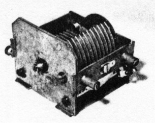
Photo A - Ordinary capacitor.
Shape of rotor plates
If the capacitor rotor plates are specially shaped, this dial compression can be spread out. In general, the radius of the rotor plates must be reduced at the minimum capacitance end so that each degree of rotation causes less capacitance change. With correctly shaped rotor plates, an equally spaced linear frequency scale results. The plates are referred to as "straight line frequency variables." Capacitors constructed this way are usually not available or very expensive. One exception is the WWII surplus capacitor described in Reference 2 and shown in Photo B.
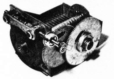
Photo B - World War II capacitor.
Worst-case dial error
Equations in the appendix of Reference 1 show how to calculate the degree of error a linear dial will have when a straight line capacitance variable is used. The frequency at the dial center will be low if the end points are set exactly. Note that the worst-case error can be reduced to one-half by setting the frequency at both ends of the dial high by one-half the center dial error. This error is shown in the graph in Figure 1, plotted as a percentage of full-range error for various frequency tuning ratios. The range is defined as high frequency minus low frequency, and the errors have been reduced to one-half.
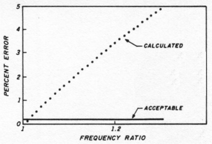
Fig 1 - Percent error for straight line capacitance variable.
The curve is very steep; the error is unsatisfactory for all but very low tuning ratios and narrow ranges. I consider an error of ±1 kHz in a 500-kHz range satisfactory and an error much beyond that as excessive. For example, the area below the dotted line in Figure 1 represents the acceptable region.
Low satisfactory tuning ratios force you to select fairly high frequencies to cover a reasonable range. In Reference 1 I chose 11.5 to 11.75 MHz to cover a 250-kHz range with a ±2-kHz worst-case error. That let me receive 3.5 to 3.75 MHz with an IF of 8 MHz.
Comparison with the curve of Figure 2 for the specially constructed WWII capacitor(2) shows that very low errors are possible for a 1.25:1 frequency ratio. Such capacitors are usable for a single ratio. However, the technique described here can be used for many frequency ratios.
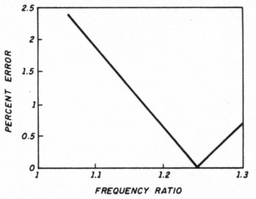
Fig 2 - Percent error for special World War II capacitor.
Eccentric pulleys
One way to reduce the capacitance change at the high frequency end is to mount an off-center (eccentric) pulley on the shaft and drive it with dial cord. The mounting must be made so the cord winds or unwinds with a maximum radius when the capacitor is at the high frequency or low capacitance end. Check the conceptual sketch in Figure 3 for details.
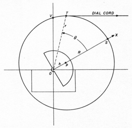
Fig 3 - Eccentric pulley.
If this pulley were just the right shape, you'd have the same effect you'd have if the capacitor plates were cut to exactly the right shape for linear frequency response. Such a pulley would be very difficult to make. On the other hand, circular pulleys are easy to make from PlexiglasTM as described in Reference 1. Note, however, that the shaft mounting hole will be off center - you can't use it in the initial turning, filing, and sanding of the rough cut pulley when it's mounted in an electric drill.
Instead, the rough cut pulley is mounted on center to a mandrel with machine screws as shown in Photo C. The off-center shaft hole is drilled after the pulley has been completed and removed from the electric drill. I realize that you may wonder how far off an eccentrically mounted circular pulley arrangement will be, and if it will be close enough to the right shape for a linear frequency scale.
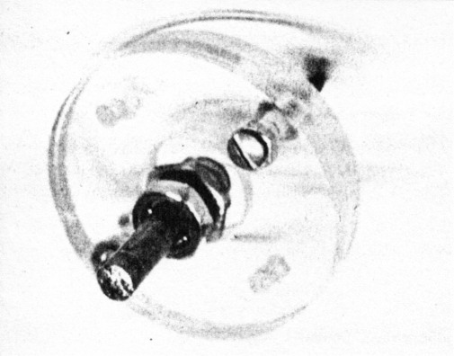
Photo C - Mandrel.
Theory
Figure 3 shows a pulley with center P and radius PS of length R. It's mounted on a variable capacitor at point O, which is length h off center. The capacitor and pulley rotate around point O. A dial cord pulls horizontally on the pulley. Note that distance r from tangent point T to center 0 changes as the pulley rotates through angle θ from 0 degrees (plates fully unmeshed) to 180 degrees (plates fully meshed).
Because the distance r changes, the amount of capacitor rotation produced by a given increment of dial cord movement also changes. This is the desired effect. Note that the point of tangency T will coincide with the vertical y axis at θ = 0 degrees and θ = 180 degrees. For other angles in between it moves slightly to the right as shown. The difference in distances OT and OV will be small and are ignored in this analysis. Mathematically, length r is given for any angle B by the following equation:
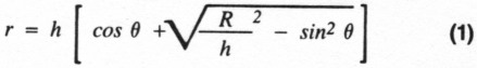
This formula is derived in the article's appendix. The appendix begins with a formula from an old high-school math textbook.(3) It's not necessary to understand the details of these equations to use this technique in Amateur construction. I've reduced the math to graphical easy-to-use results.
Finding perimeter distance TS
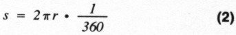
As the dial cord is pulled to the right, it unwinds from the pulley. The unwound length is perimeter distance TS. Assume the dial cord is pulled an equal amount for each increment of change in the main tuning knob and dial. This is what happens with the usual dial and tuning knob arrangement, where the dial is driven by an on-center pulley of approximate radius R/2. That is, the dial rotates through 360 degrees for a 180-degree rotation of the capacitor pulley. If you know distance TS for each angle 0, you'll know the capacitance change for each increment the dial cord is pulled, or (in effect) each increment of dial rotation.
The method for finding distance TS using numerical integration follows. I calculated the distance r from Equation 1 by taking 100 increments of θ from 0 degrees to 180 degrees for a preselected offset h. The perimeter distance traveled through a 1.8-degree increment of θ is equal to:
Each small increment s will be slightly shorter than the previous one. Add these increments of length from 0 to θ degrees for each angle θ. I now have a table of values of length TS for all 100 values of θ. I repeat the process for each offset value h. One such table is shown in the first two columns of Table 1 (for h = 0.5 R). I recommend that you use a personal computer for these calculations.
| 0 (degrees) | Length TS (inches) | Frequency F (kHz) |
|---|---|---|
| 0 | 0 | 0.1 |
| 1.8 | 0.04711 | 0.09950 |
| 3.6 | 0.09419 | 0.09901 |
| 5.4 | 0.14121 | 0.09853 |
| 7.2 | 0.18815 | 0.09806 |
| 9.0 | 0.23498 | 0.09759 |
| 10.8 | 0.28169 | 0.09713 |
| 12.6 | 0.32825 | 0.09667 |
| ↓ | ↓ | ↓ |
| 180 | 3.1416 | 0.07071 |
With the arrangement shown in Figure 3, the capacitance at θ = 0 is equal to the variable capacitor's minimum value Cmin plus any fixed external capacitance. Call the total:
![]()
As the capacitor rotates to angle 0 degrees, its capacitance increases to the following:

The frequency, however, is given as follows:
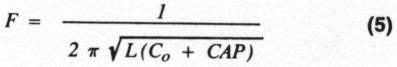
Select a value for Co (a value of external capacitance). Calculate CAP from Equation 4 and f from Equation 5 for each of the 100 values of θ in the table. Include these numbers as a third column in the table.
Frequency linearity
For a particular value of pulley offset h and a particular value of external capacitance Cexl, you now have 100 values of dial position TS and 100 corresponding frequencies. You may wonder about the linearity of the resulting frequency if you're using a linear dial like one made from a circular protractor (suggested in Reference 1). This question is best answered by drawing a best-fit straight line through the points on a graph of frequency F versus dial position TS. The deviations of the points calculated from this best-fit straight line give the error. A graph of these deviations is shown in Figure 4. I prefer to divide the error by the frequency range covered and call this the percent error. Then I plot percent error versus frequency ratio fmax/fmin.
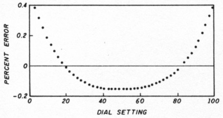
Fig 4 - Best fit deviation of calculated frequency from true straight line.
For each offset value h, you can try a range of fixed external capacitance to see which gives the lowest percent error. Note that frequency range covered, and therefore the frequency ratio, will be different for each value of external capacitance.
Frequency ratios
These data points are plotted in Figure 5 for values of offset: h = 0.05, 0.1, 0.2, and 0.5. Note that there's a range of values for each h value where the percentage error is quite low. To the left and right the error gradually increases. For larger offsets h, the minimum occurs at larger frequency ratios.
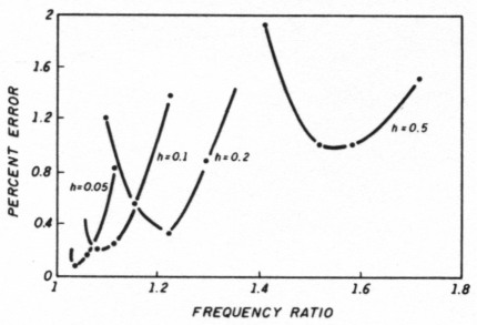
Fig 5 - Percent error as a function of frequency ratio for four offset values h. This is the main result of the calculations.
This is to be expected, because a larger frequency ratio requires a larger difference in the capacitance changes at the dial ends than a low ratio does. Larger offsets h produce larger differences in the distance r at the Cmax and Orlin ends.
Also note that the minimum percentage error is larger with larger values of h. This is undoubtedly because an off-center circle isn't exactly the right shape for a linear frequency scale. The variation from the correct shape becomes greater at larger frequency ratios.
Nevertheless, quite acceptable percentage errors are produced with the easy-to-build, circular, off-center mounted pulleys. As I mentioned earlier, I consider an error of 0.2 percent, or 1 kHz, in a 500-kHz frequency range dial very acceptable. This is about the limit at which I can set such a dial by eye, if I'm very careful.
Figure 6 shows another plot of frequency differences from a best-fit straight line with an external capacitance set for an error near the minimum. I've included this to illustrate the type of error you would normally experience because you'd usually select a deviation h and external capacitance Co for a minimum error.
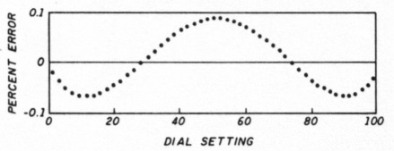
Fig 6 - Deviation with external capacitance set for minimum error.
Figure 5 is the key operating result of all this theory. You can use it to optimize any off-center tuning design. You can also see what effect small differences in mechanical dimensions or external capacitances will have. In general, because the curves are so flat near the minima, minor construction differences won't have much consequence. Small percentage errors are readily achievable as the next section will show.
Practical verification
I built an operating model to verify these results. A note on the overall dial stringing is necessary here. Any off-center pulley like the one shown in Figure 3 requires that the dial cord be returned to the pulley at the same (varying) rate it is removed. Otherwise the cord will become too loose or too tight. The simple sketch in Figure 7 won't work with this off-center pulley.
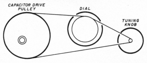
Fig 7 - Impossible arrangement.
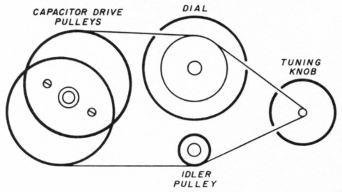
Fig 8 - Dual eccentric pulley arrangement.
Resolve the problem by using a second off-center pulley, offset in the opposite direction. Figure 8 shows an offset which has been greatly exaggerated. As the main tuning knob is rotated clockwise, the top dial cord comes off the off-center pulley and an equal amount is picked up by the other pulley from the bottom cord. You need a small idler pulley to keep the bottom cord horizontal (approximately). This is the arrangement I selected and built. It's shown in Photos D, E, and F and operates very smoothly.
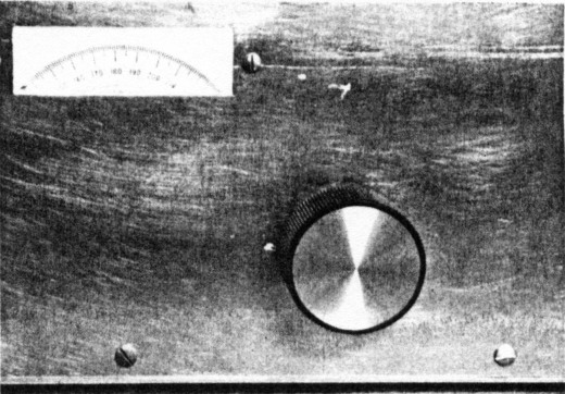
Photo D - Dial assembly, front view.
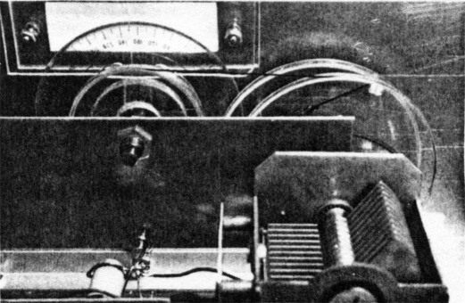
Photo E - Dial assembly, back view.
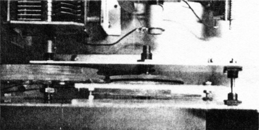
Photo F - Dial assembly, top view.
Pulley details
I completed the pulley construction using the method in Reference 1. I also built the mandrel shown in Figure 9 and Photo C using the same techniques. This mandrel holds the large pulleys on center when each is mounted temporarily to the mandrel with four machine screws. After a large pulley is shaped and the groove is cut, it's removed from the mandrel and its mounting hole is drilled off center. My large pulleys have a diameter of 3-1/2 inches. The mounting hole was drilled 0.175 inches off center for h = 0.1.
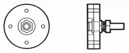
Fig 9 - Mandrel for pulley construction.
You can do this easily by marking the off-center location with an awl, drilling it with a small 1/16-inch or smaller drill, and increasing the hole diameter with gradually increasing bit sizes. The final one should be 3/8 inch. The second large pulley has its mounting hole cut for 3/4 inch with a hole-cutting attachment, like the one shown in Reference 1. This larger size lets you mount the locking shaft securely. The two pulleys are held together with machine screws. Check the photographs for details.
Pulley sizes
I mounted an aluminum front panel and subpanel on an aluminum bottom plate following the sketches in Reference 1. In this case the dimensions were as follows: Dial pulley diameter 2-1/4 inches. Dial pulley centered 2-5/8 inches above base plate. Capacitor pulley centered 2 inches above base plate. Idler pulley diameter: 3/4 inch. Idler pulley centered 11/16 inch above base plate.I cut the shafts to length, and once all were operating smoothly I strung the dial cord as shown in Figure 8. You should use a small spring at one end to keep the dial cord under tension. The arrangement is shown in Photos D (front view), E (back view), and F (top view).
The circuit
Its important to use a high quality capacitor. For my setup, I used the ARC5 oscillator capacitor1 shown in Photo A. Photo E has the details. I also used the CA3028 circuit with emitter follower buffer of Reference 1. I tried several values of fixed capacitor to establish the value needed for a 1.1:1 frequency ratio. The graph in Figure 10 shows the measured results. About 600 pF is right for the dial with its h = 0.1.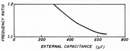
Fig 10 - Frequency ratios for various external capacitors.
Frequency readings
With the pulley directions just given, a 250-degree rotation of the circular protractor dial gives slightly less than 180 degrees of capacitor rotation. I took readings every 10 degrees from 0 to 250, then plotted and curve fit them to a straight line. Figure 11 shows the results. The less than 0.8-kHz error for a 2 to 2.2-MHz range agrees with the calculated results shown in Figure 5.
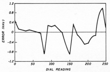
Fig 11 - Deviation of measured frequencies with 600-pF external capacitance (2.0 to 2.2 MHz).
Another check with 220-pF external capacitors is shown in Figure 12. The resulting 1-percent error also agrees with Figure 5.
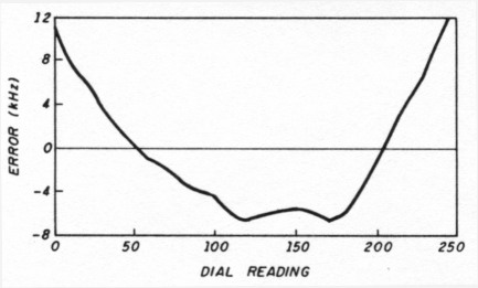
Fig 12 - Deviation of measured frequencies (2.8 to 3.4 MHz; 220 pF external).
Finally, I decided to see how well this off-center apparatus can cover the 5.5 to 6-MHz range. This is the 500-kHz range used in my Kenwood transceiver. I replaced the protractor labeling with a paper disc of new labels from 0 to 500, covering the 0 to 250 degrees on the original labels. I left the outer degree lines visible and indicated 2-kHz markings. Then I mounted an external 140-pF APC trimmer capacitor next to the oscillator coil and changed the fixed capacitors as shown in Figure 13.
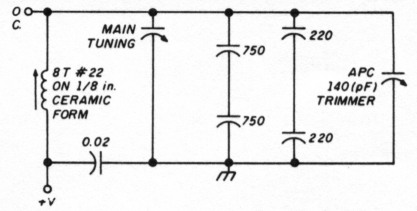
Fig 13 - External capacitors for 5.5 to 6.0-MHz range.
After adjusting the inductor for 5.500 MHz at the low end and the trimmer for 6.000 MHz at the high end, I took frequency counter readings for every 20-kHz position of the dial. Table 2 shows my results. A 1-kHz maximum error across the dial is acceptable, in my opinion.
| Dial | Frequency (kHz) |
|---|---|
| 0 | 5500 |
| 20 | 5519 |
| 40 | 5539 |
| 60 | 5559 |
| 80 | 5579 |
| 100 | 5600 |
| 120 | 5620 |
| 140 | 5640 |
| 160 | 5660 |
| 180 | 5680 |
| 200 | 5700 |
| 220 | 5720 |
| 240 | 5741 |
| 260 | 5760 |
| 280 | 5780 |
| 300 | 5801 |
| 320 | 5820 |
| 340 | 5839 |
| 360 | 5859 |
| 380 | 5880 |
| 400 | 5899 |
| 420 | 5920 |
| 440 | 5940 |
| 460 | 5961 |
| 480 | 5981 |
| 500 | 6000 |
Conclusion
I find it practical to perform near linear tuning using dual eccentric pulleys, and know of no other way to get this kind of linearity out of a straight line capacitance variable. The technique appears to be new, probably because the math required for analysis is quite involved. But by using the main result of Figure 5, you can build practical tuners easily in your home workshop.
Appendix
To derive Equation 1, start with the general equation of a circle:
![]()
This is given in polar coordinate form by Currier(3) on page 291:
![]()
For the circle in Figure 3, the x axis is as shown and the y axis would be perpendicular to it. Angle O and distance r are shown. A circle centered at x = h, y = o is given by the following equation on page 240 of Reference 3:
![]()
Value R is the distance from P to S, the true radius of the circle. Expanding Equation 8 you get:
![]()
Compared to Equation 6, A = -2h, B = 0, and C = h2 - R2.
So Equation 7 can be written for the circle of Figure 3:
![]()
Solve for r using the quadratic equation:
![]()
Using the well-known identity 1 - cos2θ = sin2θ:

Rejecting the negative value gives you Equation 1.
References
- John R. Pivnichny, N2DCH, "A Homebrew Tuning Dial." Ham Radio, December 1988. page 75.
- John R. Pivnichny, N2DCH, "Linear Tuning with a War Surplus Capacitor;" Ham Radio, June 1989, page 40.
- C. Currier, E. Watson and J. S. Frame. A Course in General Mathematics, Macmillan, New York. 1957.
N2DCH, John Pivnichny.