Receiver front-end limitations
Following on from the article on receiversensitivity, Gordon J King IEng AMIERE G4VFV now looks at the problems involved with the overloading of receiver front-ends.
Although receiver fronts-ends are low-level stages (designed to work with very low signal levels) they do exhibit some of the characteristics of high-level power amplifier stages, especially in terms of input overload. If a power amplifier ('linear') is driven hard there comes a point as the drive is increased when the rise in output fails to correspond to the increase in input. Eventually, no output level change occurs as the drive is further increased (very severe overload). Thermionic valve amplifiers generally have a more gradual lead-up to the compression point than do amplifiers based on solid-state devices. Valve amplifiers tend to overload more gracefully!
Compression is the symptom of amplitude non-linearity, which is best shown by a curve, as in Fig. 1. Here, the full-line curve represents an input/ output (transfer) characteristic. A perfectly linear transfer characteristic, as indicated by the broken line, would yield an output at C on the output axis. However, due to the compression, the output in reality rises only to point B.
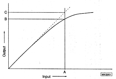
Fig. 1: Input/output transfer characteristic, showing non-linearity and ultimate compression which are responsible for r.f. intermodulation.
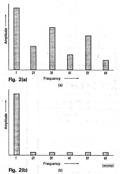
Fig. 2: (a) Harmonics to the 6th order resulting from amplitude non-linearity. (b) Very low amplitude harmonics resulting from more linear operation.
Compression in itself is not really the problem since this could be calculated for. The primary problem is the effect that the amplitude non-linearity has on the spectrum of the signal emerging from the amplifier. Let us suppose that we drive an amplifier with a signal of frequency fat input level A. Now, owing to the non-linearity and hence the compressed output, the signal at output level B might well have the spectrum as shown at (a) in Fig. 2. Here, in addition to the fundamental signal f, we have a multiplicity of harmonics at 2f, 3f, 5f, 6f, etc.
Absolutely perfect linearity in any valve or solid-state amplifier is an impossibility. Thus, there is always going to be some harmonic production. With a sanitary drive, though, so that only the most linear part of the characteristic is utilised, the amplitude of harmonics and their numbers will be very small indeed. It is only when we start driving linears' and, indeed receiver front ends hard, that nasty things happen. The spectrum at (b) in Fig. 2 would be representative of a very linear transfer characteristic. Here, only very low-level harmonics are shown.
Looking again at (a) in Fig.2, we see that the odd-order harmonics (3rd, 5th, etc.) have a higher amplitude than the even-order ones. (2nd, 4th, 6th). Whether the odds or evens are of the higher amplitude' depends essentialy on the mathematical nature of the transfer curve itself. Valves and field effect transistors have a curve which tends towards lower amplitude odd-order harmonics, while the converse is generally true for bipolar transistors.
Harmonic Effect
The production of harmonics in power amplifiers can be easily understood to be an undesirable state of affairs, since we are then transmitting spurious signals as wel as the fundamental. A 144MHz band linear, for example, driven at say 144.5MHz would produce a series of harmonics at 289MHz, 433.5MHz, 578MHz, etc. The strength of the harmonics would increase with the increase of drive to the linear. How well they would be transmitted would depend on the linear's filtering, the antenna used and, indeed, on whether any bandpass filtering is used between the output of the linear and the antenna!
The effect of receiver front end overload is less apparent, yet it can be be mistaken for a transmitter shortfall, especially on the 144MHz band under conditions of high activity. One example of this is when a strong , local signal appears on several frequencies as well as on its correct frequency. The strong signal may also appear 'mixed' with weaker signals, an effect sometimes manifest on f.m. simplex channels when many stations are working simultaneously on the band and when an antenna pre-amplifier is in use. Similar symptoms can result, of course, if the transmitter producing the strong signal is generating spurious signals - but it is usually the receiver front-end overloading rather than the transmitter producing spurii.
RF Intermodutation
In addition to the creation of harmonics from a pure, single frequency signal, amplitude non-linearity can also produce inharmonious signals when two or more signals of different frequencies are applied to the input. These new signals are called intermodulation products, IPS for short. Let us consider what happens when there are just two signals on frequencies f1 and f2. First, two new signals are produced corresponding in frequency to f1=f2 and f2-f1. As an illustration let us make f1 144.500MHz and f2 144.51MHz. Thus the new signals correspond to 289.01MHz and 0.01MHz and, in this case, are so far removed from the 144MHz amateur band that they are generally insignificant. These are called second-order IPS. In addition to these, there are also the straight harmonics of f1 and f2, such as 2f1, 2f2, 3f1, 3f2, etc., but again since these are well above the fundamental frequencies they are naturally filtered out by the circuit design.
Odd-Order RF Intermodultation
Odd-order harmonics include the 3rd, 5th, 7th etc., as we have seen. Now, odd-order r.f. intermodulation is a much bigger problem than 2nd or even-order r.f. intermodultation because the new frequencies produced can fall close to the originating frequencies, especially when the originating frequencies themselves are close together. The sum products such as 21l + f2 and 2f2 + f1 are not such a problem since, again, they are well up in frequency.
However, let us consider the 3rd-order IPS which correspond to 2f1 - f2 and 2f2 - f1 using the two frequencies for f1 and f2 as just exampled. We then find that 3rd-order IPS are produced, separated by a mere 10kHz. This is better seen from the spectrum display in Fig. 3. This display also reveals other pairs of IPS, corresponding to the 5th and 7th orders.
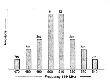
Fig. 3: RF intermodulation products arising from two parent or driving signals at f1 and f2. Each order yields a pair of products. The 3rd-order products are usually of greatest amplitude and are therefore more important than the others.
The 3rd-order products result from the product of three signals, which can either be independent signals or just two signals as we have seen. The 5th-order IPS derive from 3f2 - 2f1 and 3f1 - 2f2, while the 7th-order IPS derive from 4f2 - 3f1 and 4f1 -3f2. The even higher odd-order IPS continue in this sequence. In other words, each pair of IPS is separated evenly from its partner by a frequency equal to the difference frequency of the two originating signal.
The amplitude of the IPS depends on the amount of non-linearity involved, while the orders are influenced by the mathematical nature of the non-linearity. As already noted, valves and field-effect transistors generally produce lower amplitude odd-order IPS than bi-polar transistors, which is one reason why field-effect transistors are commonly employed in receiver front-ends.
All the IPS in Fig.3 would tend to find their way through the receiver circuits and give rise to spurious responses, assuming sufficiently large amplitudes. Remember, though, that it needs at least two signals to produce IPS, and that for significant response the two signals would need to be relatively strong. Under practical conditions, the effect on reception can change as different signals of varying strength come and go. With only one of the originating signals modulated, each response would carry that same modulation. With both modulated, however, each spurious response might well carry the modulation of the two (or more) signals.
When the modulation is single-sideband, severe 3rd or higher odd-order intermodulation has the effect of widening the bandwidth so that each signal of excessive strength appears to occupy a greater spectrum than normal. This is because an s.s.b. signal has its own range of audio sidebands, which themselves produce close-in IPS. Such apparent widening might also be accompanied by difficulty in achieving resolution of the s.s.b. signal.
When there is a multiplicity of strong signals, as there well might be under lift conditions during a contest, for example, the signals all tend to to add on a peak basis, so that ultimately the net signal level is such that even the best of of front-end designs commences to exhibit the symptoms of odd-order intermodulation. This is particularly likely when a fairly high-gain antenna preamplifier is connected between the receiver (or transceiver) antenna input. If such an amplifier has a gain over the passband of, say, 12dB, then the signal level applied to the frontend will be lifted by four times (12dB equals four times voltage ratio), which could be enough to push the receiver r.f. amplifier/mixer into severe non-linearity. Things can become pretty hectic when there are several very strong s.s.b. signals on the band, owing to the complex intermodulation of their sidebands!
Signals which are not actually within the 144MHz amateur band can sometimes evoke spurious responses, should they find their way into the front-end from the antenna at high level. For example, two very strong signals, one at 133MHz and the other at 278MHz, would produce a weak response at 145MHz (in band), even though the unwanted signals are outside the tuning range of the receiver. This would be a 2nd-order response at f2-f1 (278MHz-133MHz = 145MHz). Although the input selectivity of 144MHz transceivers is fairly flat over the band, there is generally a reasonable degree of band-pass filtering which should attenuate out-of-band signals (see Fig. 4). However, when a very strong signal falls just out of the amateur band, then it may be necessary to use additional filtering at the receiver input.
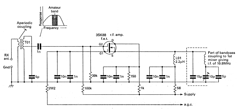
Fig. 4: The r.f. amplifier front-end of the Yaesu FT-480R, showing the aperiodic antenna coupling (fairly wideband) and part of the bandpass coupling to the mixer.
Modern h.f. transceivers are commonly equipped with a number of separate bandpass filters, providing both r.f. preselection and r.f. to mixer preselection, one set for each band, which are diode-switched. Triple or quadruple conversion is also common nowadays, with intermediate frequencies in the order of 40MHz, 9MHz and 455kHz. The high frequency first i.f. minimises 'image' responses by shifting them outside the response of the r.f. pre-selection.
IF and Image Responses
The Trio TS-940S has quadruple conversion with intermediate frequencies of 45.05, 8.83MHz, 455 and 100kHz (the latter i.f. is not used on f.m.). The oscillator in this example would be running at 59.25MHz to yield the 45.05MHz first i.f. from a 14.2MHz incoming signal. (e.g., i.f. equals oscillator frequency minus incoming signal frequency). A signal arriving at the input around 45.05MHz would have to penetrate the pre-selection of the band in use to produce a response. The rig could be expected to have an i.f. rejection ratio of, at least, 100dB, which means that an antenna signal around 14mV at the i.f. would be needed to evoke a similar response as a tuned, in-band signal of 0.1411V.
Still assuming a local oscillator signal of 59.25MHz, the mixer would also produce the first i.f. of 45.05MHz from an input signal of 104.3MHz (e.g., 104.3 minus 59.25 equals 45.05MHz). This response, which occurs at the tuned frequency (14.2MHz) plus two times the i.f. (90.1MHz), is known as the second-channel or, more commonly now, the image response. Again, the degree of response is dependent on the attenuation provided by the r.f. pre-selection at the particular band. A rejection ratio similar to that of the i.f. should be expected.
Another spurious response not very often considered, is known as half i.f. response or repeat spot response. Let us still assume that the receiver is tuned to 14.2MHz and that a very strong signal at 36.725MHz is being picked up by the antenna. This signal could be strong enough to produce a second harmonic at the front end of 73.45MHz. Now, let us also suppose that the local oscillator is producing a second harmonic at 118.5MHz. Thus, from these two signals the mixer will deliver the i.f. (e.g. 118.5 minus 73.45 equals 45.05MHz). The repeat spot, then, is produced by a strong signal which is half the i.f. above the tuned frequency, when the oscillator is working the i.f. above the signal frequency. It usually needs a very strong signal to evoke a response, the suppression ratio also being dependent on the purity of the oscillator signal.
Blocking
Sometimes called gain compression, the blocking effect is very apparent when a strong carrier occurs somewhere within the passband (often close to the signal), since then the wanted signal falls dramatically in strength, just as though the strong signal has taken away the wanted signal. Blocking is caused by a stage in the front-end being driven so hard that it becomes saturated and then has difficulty in passing any further signal (see Fig. 1). Blocking and intermodulation are somewhat related in terms of cause at least.
Reciprocal Mixing
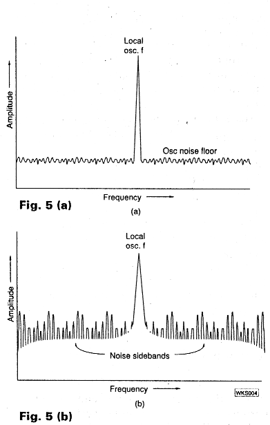
Fig. 5: (a) Spectrum of a very 'pure' local oscillator signal. (b) Spectrum of a local oscillator affected by noise sidebands. These can be transferred to a weak, wanted signal when a strong carrier occurs close to the weak, wanted signal. This is reciprocal mixing, as explained in the text.
Another large signal aberration is so-called reciprocal mixing, but unlike harmonic production, intermodulation and blocking it is not a direct result of non-linearity. Reciprocal mixing stems from the local oscillator which, instead of possessing an absolutely 'pure' spectrum, is endowed with undesirable noise sidebands. A pure oscillator spectrum would appear as at (a) in Fig. 5. Here the oscillator signal rises cleanly above the noise floor.
The spectrum at (b) shows an oscillator signal rising from a much higher noise floor which is, in fact, composed of a whole spectrum of noise sidebands, clustering each side of the signal. Fig.5 (b) is the sort of spectrum that might occur from a particularly noisy frequency synthesiser, being very similar to that of tape modulation noise.
Let us suppose that our 144MHz band rig is tuned to a weak signal at 144.3MHz, that the first i.f. is 10.8MHz and that the frequency of the local oscillator is below the frequency of the incoming signal, therefore running at 133.5MHz. If a strong signal were suddenly to appear at 144.31MHz, 10kHz above the tuned frequency, it would arrive at the mixer and, in effect, tend to act as another 'local oscillator' signal, while the sideband noise from the real local oscillator would then seem to the mixer as another 'wanted' signal.
That sideband noise centred on 135.51MHz would thus appear within the i.f. passband along with the real wanted signal. In other words, the oscillator noise sidebands would be dumped on the weak 144.3MHz signal we are trying to receive, thereby further impairing its signal and hence readability noise ratio. In a severe case the noise sidebands might completely mask the weak signal. It is because of the reversed role of the mixer to the slightly off-frequency strong signal, acting as a 'local oscillator', and the noise sidebands acting as a 'wanted signal' that the term reciprocal mixing has been coined.
One of the purest oscillators is a crystal circuit with high Q tuning. It is almost impossible to measure reciprocal mixing accurately with a synthesised signal generator, but for this test I have found the non-synthesised Marconi TF995B/2 signal generator useful. This instrument uses valves and has a relatively clean spectrum.
The parameters discussed relate to the strong signal performance of receivers, that is, how strong a signal can be accommodated before the receiver badly misbehaves. The 3rd-order intermodulation performance is very important since it can set the upper side of the dynamic range sandwich (the noise floor and sensitivity setting the lower side). Poor 3rd-order intermodulation performance will also lift the noise floor under the practical conditions of many in-band signals and sidebands. The 3rd-order response increases by 3dB each time the r.f. is raised by IdB (5th-order by 5dB per dB r.f. increase, and so on).
Intermodulation problems arise from any non-linearity, as already explained, so in the front-end the non-linearity can occur both in the r.f. amplifier (if used) and mixer. Of course, for a mixer to function it must have non-linearity to provide the i.f. from the 2nd-order product! The craft is to keep the odd-order products as low as possible, especially under conditions of strong input signals. Recent designs are focused on the attenuation of odd-order products, with a current lean towards the use of 'double balanced' mixers. For the sake of good, small-signal performance, the mixer must also have a low noise characteristic.
Testing For 3rd-Order Intermodulation
The outputs of two signal generators are combined for the least interaction and intermodulation and the signals are tuned to the particular band and spaced, say, by 10kHz. Onegenerator is switched off, and the receiver under test is tuned to the remaining signal and the levels adjusted to provide a datum response corresponding to the receiver's sensitivity. Both generators are then switched on and the receiver tuned to one of the 3rd-order responses. For example, the tuning would be to 144.490 or 144.520MHz if the two input signals are at 144.500 and 144.510MHz.
The outputs of the two generators are increased in step so that their amplitudes correspond until a response signal equal to that of the datum sensitivity response is obtained. The 3rd-order intermodulation ratio can be expressed as the dB difference between the input required for the 3rd-order response and that for the on-tune datum sensitivity.
RF Intercept Point
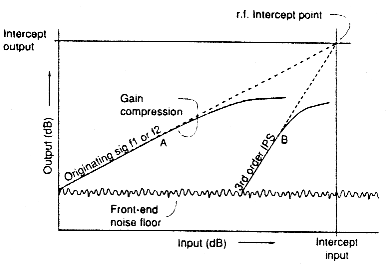
Fig. 6: A plot expressing the r.f. intercept point, which can be referred either to the input or output signal level. This is fully explained in the text.
Another expression of 3rd-order (or higher odd-order) intermodulation is shown in Fig. 6. A plot (curve A) is made of the input/output power. Initially a 1dB increase at the input will give a 1dB increase at the output. The output slows and ultimately ceases at the gain compression point, and 3rd-order IPS rise from the noise floor. A plot (curve B) is then also made of this response.
Now, the r.f. intercept point is really an imaginary one which is obtained by extending the plots A and B until they meet or intercept. The parameter can then be then be expressed either as the input intercept or the output intercept. The appropriate signal level is generally expressed in dBm (dB above 1mW) The output intercept will always be higher than the input intercept by the dB gain of the device (e.g. front-end) under test.
This theoretical expression of 3rd-order intermodulation is handy because it can also be used to determine the effective dynamic range of a receiver.
As the 3rd-order response increases fast beyond gain compression, a good test is to switch off an antenna pre-amplifier if reception is marred by intermodulation problems. If the trouble clears up it is a sure sign that the front-end is being overloaded. Sometimes, just swinging a 144MHz band beam Yagi antenna off-beam, thus reducing a powerful signal coming from a particular direction, is enough to prove whether the trouble lies in the reciever or transmitted signal!