Propagation logging
It's Easier Than You Think
Tony Hopwood has been running a propagation logging station for several years. Here he describes a very simple station which can be used to increase your knowledge of h.f. propagation.
Everyone knows that long range h.f. radio reception is influenced by daylight, the sunspot cycle and the time of year. My research to determine the relationship between the earth's electric field and solar emission using electrometers, published in PW November 1988, has shown that the ionosphere is a sensitive indicator of sunspot and solar flare emissions.
The question, still unanswered, was how sensitive are h.f. radio signals to ionospheric changes caused by the arrival of charged particles from an active sun? I needed some way of recording what was happening, and that meant a recorder of some sort.
Propagation Logger
I made a propagation logger to record short wave radio signal reception over long periods. This signal was correlated with those of other instruments designed to give an early warning of magnetic storms and possible aurora.
The specification was for a propagation logger to detect and record average broadcast signal levels between 1585MHz. One solution was to automate receiver tuning and make it cycle between those limits. The signal spectrum was then integrated by recording each cycle on a chart recorder.
The more I considered this idea, the less I liked it! The main problem, is coverage and waveband switching.
A better alternative, seemed to be an broadband r.f. amplifier, fed from a broadband antenna. My final layout is shown in Fig. 1.
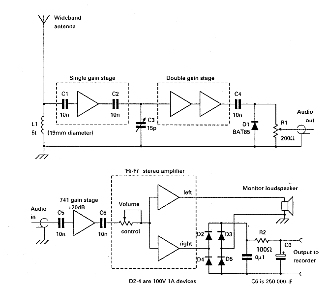
Fig. 1: The block diagram of the propagation logger. The gain stages are shown in Figs. 2 and 3.
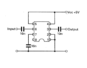
Fig. 2: The masthead pre-amplifier stage, which uses a single SL560C i.c.
The first stage, using an SL560C i.e., is shown in Fig. 2. This stage amplifies the broadband r.f. signal. The signal is then fed to a second double stage amplifier and detector. This stage is shown in Fig. 3.
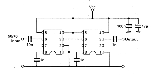
Fig. 3: Two coupled stages, as shown in the diagram, provide enough amplification before the detector stage.
Simple Plan
The approach I adopted turned out to be a very simpleplan. The SL560C can be configured to give a fairly level response from 15 to over 200MHz. So I used this version as an untuned first stage, running off a 5V supply.
The first stage was fitted in a weather-proof box, mounted on the mast of a 'fishbone' antenna. The antenna was originally built for a solar radio telescope, and designed for use on 210MHz.
The output from the first stage 'pre-amplifier' is then fed to a second double SL560 stage. This is fitted with a l5pF variable capacitor across the input, to limit the effects of the Band II f.m. broadcast band. The amplified r.f. signal is then detected by a Schottky signal diode, to provide a d.c. level output.
Amplified Audio
The d.c. output level from the logger is amplified by a 741 amplifier. This provides a signal gain of 100 to give a respectable audio signal level.
I've used an elderly pen recorder as a recording medium. The system only uses one roll of paper and a 'fill' of ink a month, but a fairly high level of signal power is needed to drive the chart recorder.
Rather than use a power amplifier i.e. stage to drive the recorder, I use an old 'Hi-Fi' audio amplifier to do the job. One output of this amplifier is fed to a loudspeaker for monitoring purposes.
The other output is fed to a power bridge rectifier, and then to the recorder. The signal, at first quite lively, was smoothed with a 250 000µF capacitor.
Fishbone Antenna
The 'fishbone' antenna design was taken from Radio Engineering. As I've already mentioned, it was originally designed for use on 210MHz.
The fishbone has a very broad response, in fact so broad that it responded to signals from 210MHz downwards. Many other antennas are featured in this book, which is written by F. E. Terman, with the maths involved reduced to a minimum.
Reception tests proved the fishbone antenna to be a good choice, although a wire antenna would work just as well.
I made the antenna and its tripod from two defunct aluminium garden clothes dryers from the local tip!
The drying cords used to pass through holes with pvc ferrules. The ferrules are on the right pitch, and they make excellent insulators for the tuned aluminium collector rods.
The rods are first cut to size. Then they are threaded with 2BA and screwed into place through the ferrules.
A carbon terminating resistor is fixed across the forward end, and 'potted' in epoxy resin to protect it from the weather. A high pass coil, L1 in Fig. 1, is then wired across the antenna end of the feed to the head amplifier. Coaxial cable is then used to connect to the masthead preamplifier.
System Response
When it was finished, I was able to tweak the system response so it covered the aircraft and I44MHz bands. But it was more by luck than design, that the system was insensitive to 85-110MHz!
The lower frequency limit of the system, seemed to be around 15MHz, which turned out to be a good compromise. A 210MHz fishbone antenna should have little response at this low frequency, so it's likely that the unbalanced feed I used, contributed to the additional h.f. pick up.
I wanted to make the most of the directional v.h.f. properties of the antenna and detect possible auroral 'lift'. So, to do this, I inclined the antenna to 45°, and pointed it to the NE to cut out local taxi p.m.r. services in Worcester and Malvem, not far from where I live.
Cacophony Instructive
When the system was on, monitoring the cacophony from the speaker also proved to be instructive! Individual stations came and went, with idents showing that the logger was picking up signals between 15MHz and the 144MHz band.
Occasionally, DX TV video field signals from the v.h.f. Band I could also be heard. At night, when the background falls to a low level, amateurs, CB operators and aircraftusing Heathrow and Luton airports (about 160km away) can also be heard.
With the system up and running, it soon became clear that the logger was producing a daily propagation curve which clearly showed the changes familiar to DXers. Data from the magnetometer and earth current recorder already show if conditions are magnetically quiet.
So, my system really helps. Now it's easy to compare the propagation profile of a 'quiet' day with the effects of a magnetic storm.
Level Rises
On a 'quiet' winter day, the signal level rises from a low night-time level at sunrise, and peaks on a level 'plateau' around 1300hrs. This continues until sunset, when it falls back rapidly to the night-time low level.
My observations and comparisons with other magnetic storms have proved interesting. They've confirmed that an aurora above the visible horizon, is signalled by a signal lift to above daytime propagation levels. This is coincident with earth current transients, and magnetometer deviation.
The logger can show when conditions are favourable by indicating a signal level above the normal daytime peak. it will also provide an audio clue as the characteristic 'round the world echo' becomes audible on some stations.
On 'quiet' nights, after the h.f. signal background drops, v.h.f. signals reflected from meteor trails also show up. So, all things considered, the propagation logger is a valuable indicator of potential DX conditions, as well as providing a practical aurora and meteor scatter early warning system.
System Refinements
Since the original system was put into service in 1987, certain refinements have been added. The refinements include a mechanical integrator, which provides a propagation count on every 24 hours for record purposes.
Organisations like the British Astronomical Association and Ron Ham's 'Propagation' column in Short Wave Magazine receive these reports.
The recordings are now integrated with a continuous multi-channel logger. This shows earth currents, electric field, low energy particle count and solar ultraviolet.
A composite recording is shown in Fig. 4. Such recordings provide an unrivalled insight into the balancing act the ionosphere carries out daily, to give a long range h.f. mirror for radio signals.
The trace shown in Fig. 4, was made on Wednesday February 17. It shows, from top to bottom, the time, earth currents, particle count, propagation, electric field stress, sunlight and ultraviolet traces.
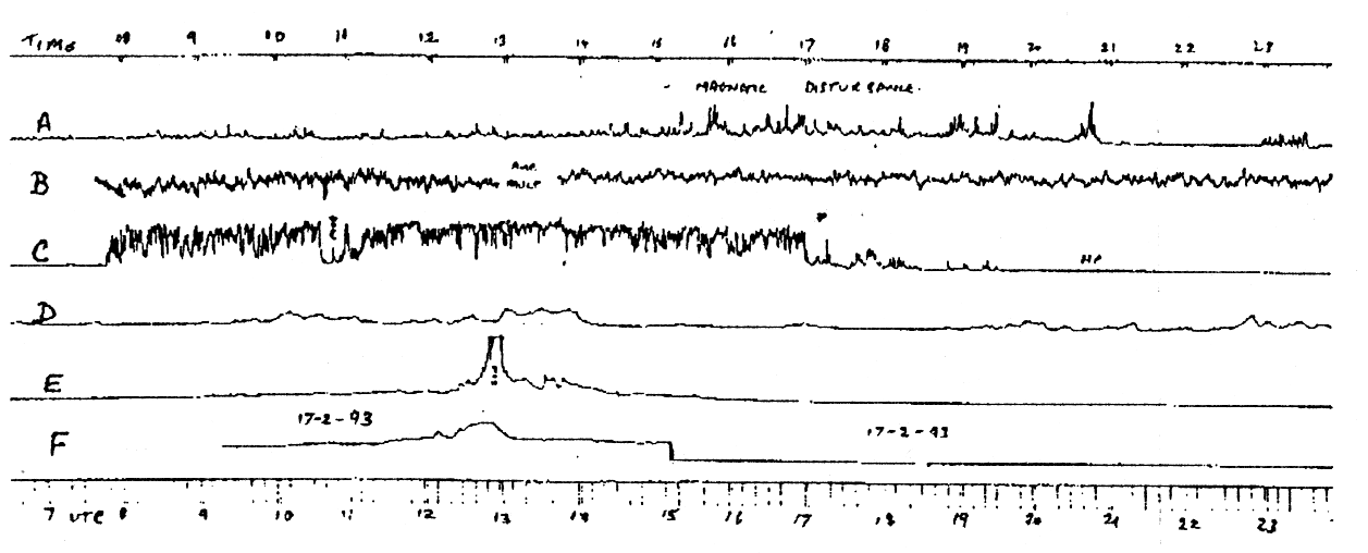
Fig. 4: The trace made on Wednesday February 17. Earth currents at A, particle count at B, propagation at C, the electric field (static) at D. Sunlight and ultraviolet are at E and F respectively.
Dellinger Fade
Interestingly, there's an almost complete Dellinger fade at about 1040hrs shown on the trace. This propagation fade, was due to an X-ray flare, which is shown as a drop on the particle count at the same time.
Later that day on the chart, there is a large magnetic disturbance. This is at a maximum at about 1600hrs, before dropping away to more normal low level by late evening.
It's also very noticeable, that around 1700hrs, the propagation conditions change to evening conditions. The vast wall of h.f. noise disappears, and by 1930hrs it's almost immeasurable.
The sunlight trace on the chart is useful. It's used to check that the ultraviolet detector is recording uv and not just bright white light.
You don't need all these different traces. I think you'll find that the propagation logger itself is a very useful item to have. So, don't just sit there! Get building and catch the DX when it arrives, not when your friends tell you about it!