More on atmospheric ozone and low-frequency propagation
Explore how LF radio signals reach your station-through chemistry and sunlight.
0zone is a trace constituent in the lower atmosphere, but it is formed after the photo-dissociation of oxygen molecules above 25 km and then carried downward by atmospheric mixing processes. Beyond that, ozone is transparent to visible light, but it shows very strong absorption in the ultraviolet (UV) part of the spectrum and is responsible for keeping harmful solar radiation from reaching the earth's surface. That absorption contributes to the heating of the "statosphere" and the rise in temperature with height in the upper stratosphere. Also, ozone is of meteorological importance as it is may serve as a tracer to show atmospheric circulation.
A recent articlel(1) pointed out that atmospheric ozone also represents a meteorological factor that affects lowfrequency and 160-meter propagation. In that study, 55.5-kHz signals were monitored daily, and the interference of the sky wave and ground wave on a one-hop path was used to show the lowering of the LF reflection region at sunrise. That transition starts from a night-time position at about 90 km, determined by the formation of negative ions in the lower D-region and goes to the day-time level below 75 km with full solar illumination.
The LF study found the transition to be delayed by about 15-20 minutes from what one would expect if visible radiation were considered responsible for detaching electrons from the negative ions at the start of the sunrise descent. That means the shadow cast by the solid earth is not responsible for the delay in the build-up of ionization in the lower D-region. Instead, the delay can be understood in terms of the opacity of the ozone layer to UV radiation and the release of electrons from negative ions that results when UV finally reaches the region with the lowering of the ozone shadow at sunrise.
This article summarizes other features that were brought out when a year-long LF study, March 1998 to March 1999, was completed. In addition, further discussion is given regarding other aspects of 160-meter propagation resulting from negative ions in the lower D region.
Experimental Details
The present study used 55.5-kHz signals on a N-S path from the Navy Station NPG at Dixon, California (38.4°N, 121.9°W) to Guemes Island, Washington (48.5° N, 122.6° W). The signals consisted of a one-hop sky wave and a ground wave. Recordings showed the result of interference between the two waves. As such, the recordings depended on the amplitudes of the sky waves and ground waves as well as their initial phase difference, while the time variations in signal strength resulted from the phase change between the two waves as the reflection region of the LF sky wave descended from about 90 km to 75 km with sunrise on the region.
The nighttime LF reflection region is characterized by a large decrease in electron density, some three orders of magnitude(2) descending from 90 km to 60 km. Of particular importance to the present discussion is the ledge between 90 km and 80 km. There the decrease in electron density is about an order of magnitude in a few kilometers, a distance less than one full wavelength (5.5 km) at 55.5 kHz. The decrease in electron density is attributed to the formation of negative ions at the lower altitudes and electrons are freed again by photo-detachment when the sun rises on the region.
Being on a small island, the receiving site was relatively free from manmade noise. There were a few instances when the recordings were not satisfactory, due to atmospheric noise as well as line noise and occasional power failures from wind storms. The records (data points every 15 seconds for about 15 minutes) typically consist of a sunrise signature, which is a decrease in signal strength, followed by a nearcomplete recovery (shown in Fig 1).
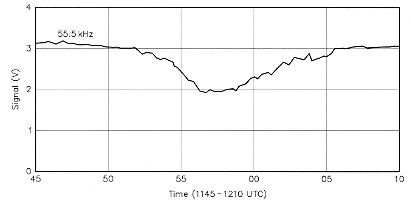
Fig 1 - Sunrise signature of NPG on June 15,1998.
The data in Fig 1 are from June 15, 1998 and illustrate the features noted above. The decrease in signal strength extended over about 15 minutes, from 1150 UTC to 1205 UTC instead of from 1125 UTC, when the start of sunrise at the 90 km level would be expected from the shadow of the solid earth. In that time, the solar depression angle at the midpoint of the path (43.45' N, 122.2' W) went from about -6° to -4° and the signal variation amounted to -2.0 dB. In the year of data recording, however, there were both faster and slower sunrise signatures, as shown in Figs 2 and 3. Those are due, in part, to seasonal differences in the rate of change of the solar altitude seen at D-region heights. Over a year's time the signal-strength variations at sunrise ranged from -0.4 dB to -3.7 dB, with an average of -1.3 dB.
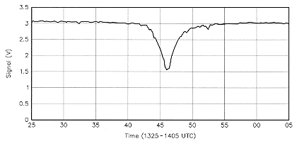
Fig 2 - An example of a fast sunrise signature on October 2,1998.
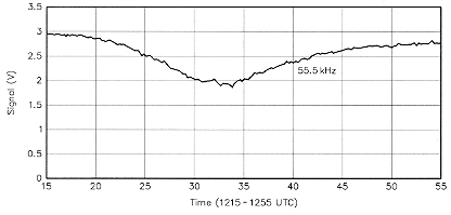
Fig 3 - An example of a slow sunrise signature on May 7,1998.
Interpretation
As noted above, the timing of the sunrise signatures can be understood from the ozonosphere controlling the time when the LF reflection region is lowered with sunrise. Turning to details of the interpretation, the vertical distributions of ozone discussed in the literature are quite varied, ranging from those having a well-defined peak to others, on occasion, with a broad, flat maximum. For the present discussion, the form of a Gaussian function was used as a reasonable representation of the ozone distribution (see Note 2). It assumes a maximum density at a 25-km altitude and a standard or mean-square deviation of 10 km from the location of the peak value. Thus, from the known properties of the Gaussian function, 68% of the ozone content would lie within ±10 km (1.0 standard deviation) of the peak of the ozone distribution. By the same token 95% lies within ±20 km (2 standard deviations) of the peak of ozone concentration.
The total ozone content in a vertical column of 1 cm2 cross-section can be expressed in terms of the thickness that the layer would occupy if the pressure and density were reduced to standard values (NTP) throughout the layer. The meteorological unit is termed a Dobson, 0.001 atm-cm, and 300 DU (Dobson Units) corresponds to an ozone layer of 3-min thickness. In that regard, the annual variation of the ozone content at midlatitudes(3) ranges from about 365 DU in the spring to 285 DU in the fall, with an average of about 325 DU. In addition, it should be noted that the deviations of daily values of ozone content from the monthly means have been observed(4) to be both large and striking.
For the matter at hand, the ozone content in the average vertical atmosphere is sufficient to block solar UV below 300 nm wavelength from reaching ground level. That being the case, an ozone column along an oblique line of sight, from the sun to the LF reflection region, was considered to be opaque to solar UV if an integration of its density along the line of sight gave a content equal to that for a vertical atmosphere (325 DU). That method was used to examine the role of atmospheric ozone by using the Earth and a spherical ozone layer, along with a straight-line solar-ray path penetrating the ozone layer, as in Fig 4. While not to scale, the figure illustrates how ray paths pass through different densities and regions in the distribution, depending on the distance of approach of the ray to the earth.
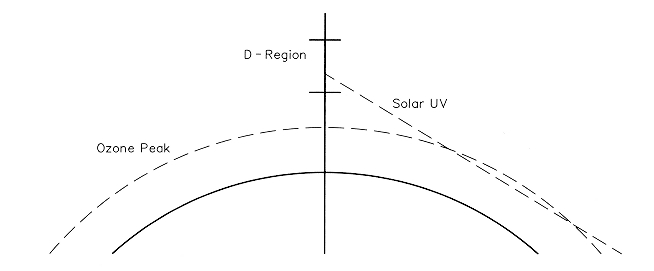
Fig 4 - illustration (not to scale) showing solar UV blocked from the
D-region by the ozone layer.
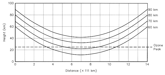
Fig 5 - Solar-ray paths at 71 solar depression when transformed to plane geometry. The height for peak ozone density is given by the horizontal line.
The same physical situation may be represented in plane geometry by transforming the straight ray paths to curved paths relative to a plane ozone layer and in 111-kin steps along the earth's surface. One example is given in Fig 5; that figure is for ray paths to the 90-km level, the altitude where sunrise starts at the midpoint of the path for NPG signals. It shows changes in the ray paths for solar angles going from -10° to -4° relative to the horizon, corresponding to the advance of time to-, ward ground sunrise (0°).
The only detail of the ozone layer given in that figure is a horizontal line at the height of the peak, taken as 25 km altitude and extending over a considerable horizontal distance. The figure also shows how the ray paths cross the level of peak concentration along the horizontal extent of the distribution. The sunrise effects are better understood if a more detailed, schematic representation of the ozone distribution is used, as shown in Fig 6. There, the diagonal pattern shows where the bulk (68%) of the ozone layer is located, at altitudes between 15 and 35 km. The two other regions with a vertical pattern are more-dilute portions of the layer, and each includes about 14% of the layer.
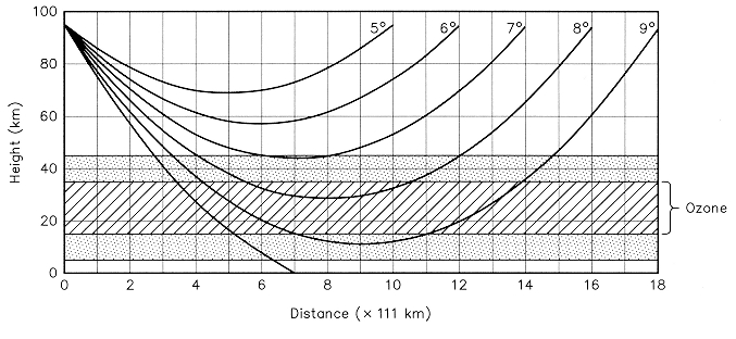
Fig 6 - A more detailed, schematic representation of the ozone distribution. The diagonal pattern shows where the bulk (68%) of the ozone layer is located, and the two other regions each include about 14% of the layer.
Like Fig 5, Fig 6 shows the ray paths for solar depression angles going from -10° to -4° toward sunrise (0°). The short ray path for -10° is given without markers in the figure and is blocked by the earth at about 777 km from the left of the figure. The other ray paths are later in real-time, with paths for -9° to -8° passing through the denser portions of the ozone layer while the path at -7° goes through the more-dilute portions of the ozone layer. Similar figures for 80 km, 70 km and 60 km show the same features, except that the paths that pass through the more-dilute portions of the layer are later in time (corresponding to angles of -6° and -5°, respectively) and the distances of closest approach to the Earth are shifted to the left of the figure by 111 and 222 km, respectively.
At this point, it is important to notice that in addition to the daily sunrise signatures, roughly 10% of the days showed other significant signal changes about 15-20 minutes before the peak of the daily sunrise signatures. Those signal variations were faster than typical sunrise signatures, taking about two minutes to reach peak values and decaying in a comparable period. The size of the variations ranged from being just detectable to -2.2 dB and, on occasions, they were sometimes noted on successive days. In addition, their distribution in solar- depression angle ranged from -7° to -8°, with an average of -7.5°, as shown in Fig 7. A typical example of a precursor is shown in Fig 8, and a precursor in association with its own sunrise signature is shown in Fig 9.
In regard to their magnitudes, they were comparable to longer events attributed to the lowering of the LF reflection region by photo-detachment and are presumed to be of the same origin.
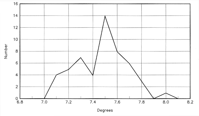
Fig 7 - Distribution of the solar-depression angles for precursor events.
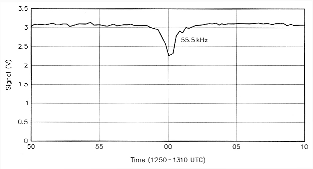
Fig 8 - A typical example of a precursor event.
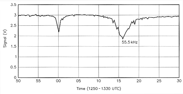
Fig 9 - Sunrise signature of NPG on September 7,1998 showing a precursor and main signature.
Ozone Distribution
Earlier, Reid(5) questioned whether the ozone layer played a role in sunrise/sunset variations of ionospheric absorption during Polar Cap Absorption (PCA) events. There, extensive calculations were carried out and ultimately showed that photo-detachment of electrons from the negative ion of molecular oxygen, in conjunction with the shadow of the Earth, could not account for the variations in absorption. After that detailed, exhaustive analysis, it was left that another ion (with a larger electron affinity and requiring UV light for photo-detachment) was probably involved and was an ion with which the ozone layer would play a major role in the day/night variations.
The present LF observations also show that the shadow of the Earth is not involved in the sunrise variation of conditions in the lower D region. That is quite evident from the fact that the sunrise signature of NPG signals is about 15-20 minutes later than would be expected from solar radiation being blocked by the solid Earth. Instead, it is possible to account for the delay just by using the known properties and extent of the ozone layer. That shows again, as Reid (Note 5) demonstrated, that the negative ion of molecular oxygen is not the controlling negative ion in the lower D region as atmospheric ozone is transparent to visible radiation.
At this point, consideration should return briefly to the precursors noted earlier, as in Fig 7. Some 39 of those events were observed during the yearlong recording of LF sunrise signatures. The very limited spread of solardepression-angle values is rather remarkable when one considers that it was obtained while observing the effects of radiation controlled by the properties of a fluid medium, not the hard, sharp boundary of the solid Earth. The question then becomes just how that sort of result is obtained and the answer proves to be both simple and complex.
Sunrise on the region of interest begins around 90 km and illumination proceeds down toward the lower D region. As shown by the ray paths in Fig 6, sunrise at the 90-km level is blocked until the ray paths for solar UV reach the outer fringes of the ozonelayer at an angle of about 70 below the horizon-for the ozone distribution used there. That goes a long way to explain the range of solar depression angles of precursors in Fig 7.
Once started, though, precursor signal variations do not continue on the path to become early examples of LF sunrise signatures, like those in Figs 1 through 3. Instead, they end after about the same time interval as it takes them to appear. Since the ray paths in Fig 6 move upward with the advance of time, there was a brief time interval during which photo-detachment took place. Then UV radiation could get through the dilute, upper parts of the ozone layer, but after that, ozone again blocked UV from reaching the reflection region.
The time when UV first got through the top of the ozone layer could have involved lower-than-normal ozone concentrations there, either a fluctuation of spatial or temporal origin. Of course, with the data in hand, it is not possible to decide which of the two was involved. The ray paths in Fig 6 show that a precursor requires a lower-than-normal ozone density in a bubble or tunnel over several hundred kilometers at the top of the ozone layer. The small number of precursor events in a year's time indicates the probability of that circumstance occurring. Nonetheless, the limited range of the solar angles during precursor events suggests that the extent of the vertical distribution of ozone used here is fairly common.
Beyond the question of vertical extent, a static ozone distribution over the horizontal distances in Fig 6 is quite unrealistic. Spatial and temporal variability of the layer, noted earlier, over that vast expanse could well be the reason why the LF precursors end after their brief appearance. In any event, vertical motions of ozone at the top of the layer seem more reasonable than horizontal motions as that transport is part of the circulation pattern that distributes ozone in the atmosphere.
Negative Ions
The discussion up to this point has dealt with the effects of ozone (a minor constituent of the atmosphere at low altitudes) and how it casts a shadow on the lower D region at sunrise. The delay in lowering the LF reflection region cited earlier indicates that visible radiation, blocked by the shadow of the Earth, is not responsible for the detachment of electrons from the negative ion population. In terms of ion species, that means that the negative ion of molecular oxygen, a constituent in the D and E regions, is not involved to any extent. Its electron affinity is too small (only 0.45 eV), and electrons would be detached with the arrival of quanta in the infrared and visible portions of the spectrum.
While there is a large body of knowledge about positive ion reactions in the D region, the same is not true of negative ions. Earlier, the negativeion reactions of oxygen species in the atmosphere were the starting point of discussions of absorption in PCA events.(6), (7) Thus, it was thought that negative ions were formed in the D region by the attachment of electrons to different forms of oxygen:
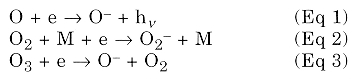 The second reaction is a three body process and M is a neutral constiuent either N2 or 02, with differen rate coefficients for each possible collission partner (see Note 2).
While photo-detachment dominates during daylight, there are different types of collisional detachment that operate day or night:
But Reid (Note 5) was unable to show the importance of negative ions of molecular oxygen in the sunrise and sunset variations of PCA events. With that, the discussion becomes more speculative, moving toward other reactions between those negative ions and the various minor atmospheric constituents such as O3, CO2, NO and H.
While ozone is formed above a 25-km altitude by chemical reactions that follow the photo-dissociation of molecular oxygen, it is then carried downward by atmospheric mixing. It then becomes part of the mixture of gases that result from human activity at lower altitudes. That same mixing carries upward carbon monoxide (CO) emissions from automobiles, nitrogen compounds from the extensive use of chemical fertilizers and water vapor from evaporation of the oceans. In the presence of solar radiation, those chemicals could be the basis from which more complex negative ions develop and populate the D region. Any greater electron affinity, up to 4.5 eV, would go to help understand the UV and ozone effects noted in the LF monitoring at sunrise.
Sunset
In spite of that statement, there remain problems with the negative ions in the D region and, more importantly, how they affect propagation at low frequencies and the 160-meter band. In specific terms, the present study was extended from the sunrise hours to those around sunset, looking for similar effects on LF propagation from the ozone layer. Thus, at first glance, it was thought that since the ozone layer delayed the onset of absorption at sunrise, perhaps it would do just the opposite: speed up the decrease of absorption with sunset. With LF observation intervals at sunset similar to those at sunrise, though, sunset signatures were just not found in number and amplitude comparable to those at sunrise. That calls for some explanation, and it must be given in terms of photo-detachment of negative ions in the D region.
About the only conclusion that can be reached at this time is that there is a continuous variation in the types of negative ions in the lower D region after the sun sets. Thus, the negative ions present at sunrise are the result of long hours of darkness, while the negative ions that form after sunset follow hours of sunlight on the region.
Therefore, the negative ions at sunrise have enjoyed many hours of darkness in which to develop. Negative ions at sunset are not quite as fortunate; they have to start from scratch as the sun goes down. Nevertheless, they do develop, mainly as atomic oxygen converts to ozone after sunset. So there is a period of growth and change after sunset, starting negative ions on reaction chains that ultimately lead to the sunrise ionosphere.
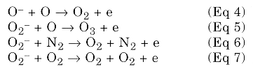
The operative word in that last sentence is "change". Nowadays, the negative ions that develop after sunset are thought to result from ion chemistry involving the minor constituents noted earlier-ozone, carbon dioxide, nitricoxide and hydrogen from water vapor. Those molecules can combine with the simple negative ions of oxygen after sunset and develop into bicarbonate ions (HCO3-) and nitrate ions (NO3-) which hold their electrons closely. Fig 10 illustrates a detailed view(8) of negative ion reactions that remove electrons from the D region with the aid of those minor constituents in the atmosphere.
Fig 10 - Schematic diagram of negative-ion reactions (after Reid, Note 8).
The left-hand side of the figure can be considered as the start (at sunset), with electrons attaching to molecular oxygen and ion reactions then proceeding toward the right-hand side, ultimately giving the stable ions in the dawn ionosphere. The progress through that complicated chain of reactions depends on the local availability of those minor constituents, from the exhaust of autos, use of nitrogen fertilizer and water vapor from the oceans and lakes.
Close examination of Fig 10 shows the various steps in which O3, CO2, NO and H are involved. However, their actual availability is dependent on the vertical and horizontal transport processes in the atmosphere. Thus, ion progress (from left to right in Fig 10) may be subject to bottlenecks when a minor constituent is missing, say a low density of ozone or nitric oxide, here or there, now and then.
All that means that the lower ionosphere, where 160-meter propagation takes place, is not a uniform region. Indeed, going from the sunset terminator to the sunrise terminator, the slow development of the negative ions which hold electrons closely will have ramifications for low-frequency and 160-meter propagation.
For that set of circumstances, negative ions species changing from one with a low electron affinity at sunset to another with a large electron affinity at sunrise, collisional detachment of electrons at sunset would yield a significant electron population in the D region. Thus, any strong gradient in electron density associated with the presence of negative ions would be absent initially. Only as atomic oxygen decays with the halt of photo-dissociation of O2 would large numbers of negative ions begin to form, albeit slowly, and then change the height of the reflection region by electron attachment.
Any changes in LF or VLF propagation that result from the rise of the reflection region would be slow at sunset, in contrast to the rapid changes at sunrise from the photo-detachment that requires UV. In that regard, a good illustration is seen in Fig 11, after a figure in Davies' book(9) (1989), where the diurnal phase changes of NBA VLF signals from Panama were observed in Boulder, Colorado. The change in phase around sunset is much slower than that at sunrise and that asymmetry can be attributed to differences in the electron affinity of negative ions in the two regions.
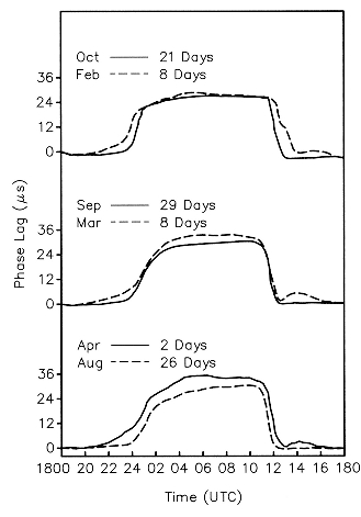
Fig 11 - Diurnal phase changes of NBA VLF signals from Panama, as observed in Boulder, Colorado (after Davies, Note 9).
160-Meter Propagation
For 160-meter propagation, absorption in the D region is the biggest concern and a growing concentration of massive, negative ions there, with a large electron affinity, serves to lower its electron density and reduces the absorption of any waves passing through the region. The question then is how rapidly after sunset does the more-stable negative-ion population develop along a radio propagation path? Experimentally, that could be estimated from absorption of a 160-meter beacon's signals from sunset to sunrise.
But leaving time or distance scales out of the discussion for the moment, one must consider the propagation mode in effect and the number of D-region traversals and ground reflections that are involved. To the extent that conventional Earth-ionosphere hops take place along a path, absorption effects would be less on anywave traversals of the D region, which are closer to the sunrise terminator than those closer to the sunset terminator, where ionospheric electrons are held less strongly by negative ions. This leads to yet another circumstance, in addition to signal ducting,(10) which favors propagation on paths going from west to east. Beyond that geographical consideration, it should be noted that the concentrations of minor neutral constituents that are involved in negative-ion chemistry, such as ozone, carbon dioxide, nitric oxide and hydrogen, are highly variable. That is the case as they are created and destroyed in various regions and are linked to circulation through vertical and horizontal transport in the lower atmosphere. Thus, like the delay in absorption at sunrise due to the role of ozone (see Note 1), there will be some variability in the electron/negative-ion distribution along a dark path, and ionospheric absorption will be quite variable as well. As a result, the meteorology of minor atmospheric constituents is seen to play an important role in 160-meter propagation.
More on Atmospheric Ozone
Concerning the meteorology of minor atmospheric constituents, their concentrations are not measured as frequently nor as widely as the other atmospheric parameters, say temperature and pressure. But in the present instance, where the reflection region of NPG's signals is lowered as UV penetrates the ozone layer, it is possible to use NPG as a beacon of sorts, looking at daily data, to examine spatial and temporal features of ozone where nothing else is available.
It should be noted, however, that the parts of the ozone layer in question are several hundred kilometers east of the path midpoint. In addition, solar directions change with the time of year, being more northerly in summer and southerly in winter. With that caveat, the results of the year-long study of LF signals can be used to look at ozone variations as well as their implications for 160-meter propagation and considered as new, fresh information.
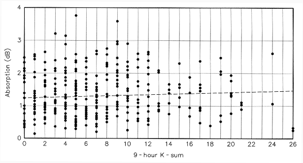
Fig 12 - Point scatter-diagram for NPG signals and 9-hour Kp-sums from records of NOAA magnetometers.
In that regard, the basic data are the magnitudes (in decibels) of sunrise signatures, the times of greatest decrease in signal strength, the corresponding solar-depression angles at the path midpoint and the shapes of the signature curves. The distribution of magnitudes of sunrise signatures is shown in Fig 12, along with the line representing a linear regression of the data. For 353 data points, the maximum and minimum values for the sunrise signatures were 3.76 and 0.2 dB, respectively, while the median value was 1.23 dB with a standard deviation of 0.69 dB. The distribution of the data points relative to the regression line do not suggest any strong correlation and the statistics bear out that point, the correlation coefficient being only 0.22.
The solar depression angles were calculated for data points above the average value, the aim being to use observations where a time could be obtained without too much in the way of uncertainty. That was not always the case as shapes of the signatures varied throughout the year and time data were not always accurate enough when the signatures were broad. But for observations where times and solar-depression angles were readily obtained from those data points above the average value in Fig 12, the distribution of angles is given in Fig 13.
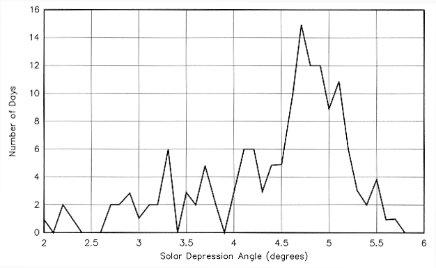
Fig 13 - Distribution of solar depression angles.
The curve shows a strong peak just below 5°, as well as a broad range of depression angles down to about 2°, but that is a summary figure for the year- long period of the study. A more informative display of the year's data is given in Fig 14, where highest and lowest depression angles are given for each week throughout the year. That figure shows a seasonal dependence for depression angles, greater angles between mid-March and mid-November than for the rest of the year.
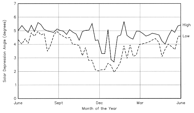
Fig 14 - Weekly values of solar depression angles.
While depression angles were smaller in the winter, the variability of the data points was much greater during winter than in summer. In particular, the spread of data points in winter was about ±1.0°, compared to ±0.5° in other parts of the year. In addition, the trends in Fig 14 are more indicative of the heights reached by the upper parts of the ozone distributions. Thus, the small angles and greater variability in winter months are characteristic of distributions of ozone where the upper part extends to greater altitudes than those with larger angles and less variability in summer.
The time durations of the sunrise signatures for the LF signals also differed with season, being longer in summer than in winter. In addition, there were differences in the shapes of the sunrise signatures. Thus, there were three distinct shapes: one with a symmetrical decrease in signal strength with time and two different, asymmetric shapes. One where the signal strength decreased slowly at first, but then with a faster recovery; and the other just the opposite, with a fast decrease and a slow recovery in signal strength.
From mid-March to mid-November, the shapes noted most often were either symmetrical or with a slow recovery, only a few having a slow onset. The asymmetric shapes with a slow onset were found more frequently in the winter months, when the spread in depression angles was greater, but a few of those shapes were also noted in the summer. Those few, however, were rather striking. They involved large changes in the depression angle, from fairly steady background values around 5° and going down to 3.0° or 3.5°, meaning there were sudden increases in heights reached by the upper parts of the ozone distributions. A search of historical weather data failed to indicate any obvious causes for those changes, though.
An effort was made to better understand the shape and the qualitative features of the sunrise signatures by using model calculations for the ozone layer. Thus, a Gaussian height distribution of ozone like that used earlier (see Note 10) to interpret the delay in sunrise signature was extended, beyond just its opacity due to the total mass of the ozone, to now include the exponential absorption of UV along the line of sight from the sun.
For that calculation, the absorption coefficient of ozone(11) was considered over the UV range, where the principal photo-detachment of negative ions would be expected. There, the absorption coefficient peaks at 140/cm-atm at 255 nm, between low values at 200 nm and 300 nm, and has an average of 75/cm-atm.
In the model calculations, the height of the peak ozone concentration ranged between 20 and 35 km. The width or standard deviation of the Gaussian distribution was varied from 6 to 12 km, and the total ozone content of the distribution taken from 0.24 to 0.36 cm-atm. With those ranges, calculations for D-region heights showed that the intensity of UV during sunrise was far more affected by changes in the height or width of the ozone layer than the total ozone content.
In regard to the last point, the total ozone content at middle latitudes in the northern hemisphere (see Note 2) shows a maximum in March of about 460 DU and drops to a minimum of about 280 DU in November. A longterm study of total ozone cited by Craig (see Note 3) shows that same annual variation but variations from monthly means that were rather large in January through March and then declined, becoming much smaller from June through November.
It is interesting to note that the weekly values of solar-depression angles in Fig 14 are more in phase, as it were, with those variations of monthly means of total ozone content than the ozone content itself. Of course, the data in that figure is only from one year of observation. Another year of study is now in progress, and it will be interesting to compare results between the two years and the variability of total ozone content.
As for the shapes of the signatures, they depend on the rate of phase change between the sky wave and ground wave as the reflection region is lowered at sunrise. The lowering results from solar UV that gets to the D region at the midpoint of the path by advancing closer and closer, as in Fig 5, through the upper reaches of the ozone layer. So the more ozone encountered, the slower the lowering and vice-versa.
With that, those signatures with more rapid change in signal strength at the outset represent cases where the top of the ozone layer was either lower or more dilute at far distances, when first encountered by the rising solar UV, than in close to the midpoint, when last encountered. By the same token, slow changes in signal strength represent cases where the top of the ozone layer was either higher or more dense at far distances than in close to the midpoint. Those signatures have implications for the onset of photo-detachment of electrons and ionospheric absorption, but it should be stressed again that they are more sensitive to the height and width of the ozone layer than the total ozone content at points along the optical path.
Conclusion
The study of LF propagation at sunrise and sunset has shown that atmospheric ozone, and probably other minor constituents in the atmosphere, play an important role in negative-ion formation in the lower D region. While the data presented here is limited to those two extremes in a day, it seems fairly clear that the lower D region is not uniform in its properties at night. Thus, the present results suggest that a significant electron density, which contributes to ionospheric absorption of 160-meter signals, is present after sunset takes place. Nevertheless, the transition to the time around dawn, when negative ions play a more important part in removing free electrons from the D region, may be variable. Moreover, it may not be predictable, given the role of transport processes in distributing minor atmospheric constituents.
While transport processes play a major role in the global distribution of ozone, notice that the brief precursor events, as in Fig 7, probably reflect such processes, but on a smaller scale. Of course, satellite measurements such as those from the Solar Backscatter UV (SBUV) detector give data for ozone profiles on a global scale; but, because of its rapid motion, the satellite cannot observe brief events in the ozone density. That problem has existed before in high altitude research, satellites often miss details of geophysical phenomena that near-stationary vehicles, such as high-altitude balloons, are able to detect. By that token, the present study using radio propagation provides a type of information about the ozone layer that is not available from any other source at the present time. The area of concern is at altitudes too high for balloons, too low for satellites and the phenomena are too infrequent for the use of sounding rockets.
Turning to propagation on the 160-meter band, it's of great interest in the winter months. In that regard, the LF signatures with lower solar-depression angles as well as greater variability in angles, noticed in connection with the data in Fig 14, suggest that ozone effects on ionospheric absorption at those times can be quite pronounced. They may actually be more variable than suggested earlier (see Note 1), before 1998-1999 winter data was in hand. It will be interesting to compare that aspect of these observations with the results from a study of dawn enhancements in the MF frequency range (Hall-Patch, private communication).
Finally, the present study was conducted in the period from April '98 through March '99. Considering that the weather patterns in that year were highly influenced by the El Niño/La Niña processes, the question arises as to whether the variability of ozone effects in the winter months between the equinoxes are typical or, perhaps more likely, reflect the unusual circumstances of the times. In that regard, an attempt will be made to obtain another year of LF data to provide an answer to that question.
Notes
- R. Brown, NM7M, "Atmospheric Ozone, a Meteorological Factor in Low-Frequency and 160 Meter Propagation", Communications Quarterly, Spring 1999, Vol. 9 No. 2, p 97.
- A. Brekke, Physics of the Upper PolarAtmosphere, (New York: Wiley and Sons, 1997).
- R. Craig, The Upper Atmosphere, (San Diego: Academic Press, 1965).
- M , Salby, Fundamentals of Atmospheric Physics, (San Diego: Academic Press, 1996).
- G. Reid, "A Study of Enhanced Ionization Produced by Solar Protons during a Polar Cap Absorption Event", Journal of Geophysical Research, 1961, Vol. 66, p 4071.
- D. Bailey, "Abnormal Ionization in the Lower Ionosphere Associated with Cosmic-Ray Flux Enhancements", Proceedings of the IRE, 1959, Vol 47 p 255,
- R. Brown, and R. Weir, "Ionospheric Effects of Solar Protons", Arkiv for Geophysik, (Royal Swedish Academy of Science, 1961), Bd. 3, Nr. 21, p 523.
- G. Reid, "Ion Chemistry of the D-region", 11 Advances in Atomic and Molecular Physics Vol. 12, (San Diego: Academic Press), 1976.
- K. Davies, Ionospheric Radio, (London: Peter Peregrinus, Ltd, 1989).
- R. Brown, "Signal Ducting on the 160 Meter Band", Communications Quarterly, Spring 1998, p 65.
- R. Whitten and 1. Poppoff, Fundamentals of Aeronomy, (New York: J. Wiley, 1971).
NM7M, bobnm7m@cnw.com