160 meter Propagation: Unpredictable Aspects
Are you likely to work 160-meter DX today? It's very difficult to say. Come learn why.
The sun is the main driving source of the ionosphere, through its ultraviolet(UV) radiation, which illuminates an entire hemisphere. A specific force is the solar wind, which interacts with the outer reaches of the geomagnetic field to form the magnetosphere. The geomagnetic field, however, is a major factor in organizing the ionosphere at lower altitudes. It controls the motions of ionospheric electrons on release by photo-ionization; and by its configuration, it shapes the global distribution of ionization, particularly at low latitudes.
The nighttime ionosphere results largely from geomagnetic control of ionization that remains after sunset, because of its low rate of recombination at high altitudes. There is also a forcing factor from the intermittent occurrence of aurora, with magnetospheric electrons accelerated to high energies going down the high-latitude field lines; those create ionization at E-region altitudes. At lower latitudes, F-region ionization decreases at night, but is maintained at low levels between the E-region and F-region peak because of UV in starlight, galactic cosmic rays and solar UV radiation scattered by the geocorona.
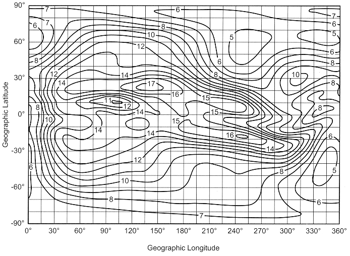
Fig 1 - Global W2 map for 0600 UTC, March 1979. (SSN-137, after Davies, Note 9).
Communication on the upper-HF bands of the Amateur Radio spectrum is largely under direct solar control. Propagation predictions are made using refraction calculations based on global ionospheric maps for the F and E regions, as in Figs 1 and 2. The F-region map shows geomagnetic control by the fact that the critical frequencies foF2 from the ionization are asymmetrical with respect to the geographic equator at the equinoxes. Also, there is the unusual distribution of critical frequencies in the F region, which shows that ionization extends into the hours of darkness at low and equatorial latitudes.
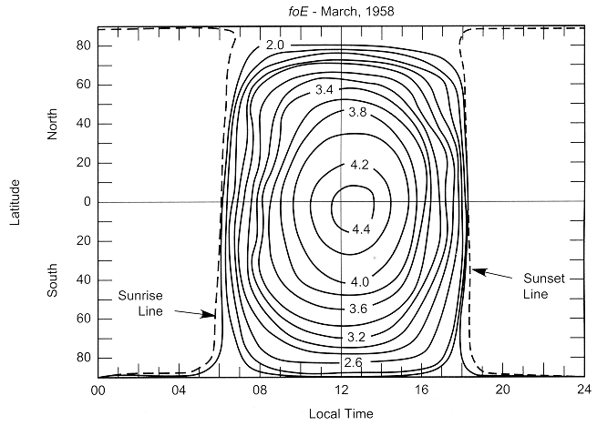
Fig 2 - Global foE map at local noon, March 1958. (SSN-201, after Davies, Note 9).
Fig 2 shows the daytime critical frequencies that result from the distribution of ionization about the sub-solar point at E-region altitudes. That is of little consequence to propagation on the higher bands of the spectrum, as the operating frequencies there are large compared to the critical frequencies foE, as well as the electronneutral collision frequencies Fc. The result is that signals go through the E region with little deviation and only small amounts of ionospheric absorption along their paths.
All in all, HF propagation can be dealt with using only a few parameters: the sunspot number or a suitable surrogate, the planetary geomagnetic K-in-dices or their short-term estimates and the announcements of bursts of solar and magnetic activity. The first two of those parameters essentially give what can be expected on average and the update material provides additional guidance when conditions depart significantly from predicted averages.
The situation is quite different on the lowest band of the Amateur Radiospectrum, 1.8-2.0 MHz. There, signals propagate at altitudes around the E region, but operations occur only at night because of the heavy ionospheric absorption during daytime. Beyond that, there is more than enough ionization overhead to propagate signals in that frequency range, so critical frequencies or MUFs-so important at the top of the HF spectrum-are of no concern. Instead, signal propagation is considered limited largely by absorption and noise.
Even at the solar minimum, sunspot numbers are sufficient to guarantee propagation on the lowest band of the spectrum. There are second-order effects that result from the sunspot number: A small increase in the radiation angle that RF must have to penetrate past the E region to permit longer F-hops and ducting. In addition, there is a small increase in D-region ionization, which increases ionospheric absorption. Both of these effects are quite within the realm of prediction and thus are easily understood and dealt with.
Nonetheless, consideration of average parameters is something of an oversimplification of the situation, as it does not recognize various propagation modes possible at low frequencies for given parameters. They, in turn, can be affected by the dynamics of the neutral atmosphere. So, with propagation being a geometrical affair, rays are refracted as they travel through the ionosphere and anything that affects the geometry of ionospheric regions relative to the earth will have an impact on signal modes.
In that regard, the phrase "relative to the Earth" has a lot of meaning as the atmospheric motions are relative to the Earth, while the ionizing radiation comes from well outside the propagation region-say, auroral electrons spiraling down relatively fixed magnetic-field lines, or solar photons on their straight-line paths from the distant sun. Thus, the level of ionization is more related to the amount of matter traversed by the incoming radiation and the neutral density, as distinct from geodetic altitude.
The atmosphere, being a target for such radiation, will present a different geometry relative to the Earth's surface for wave refraction as air parcels in the target region are moved about by highaltitude winds. Those can be seen in the motions of visible trails and radar reflections from meteors, or expected from heating and vertical expansion of the atmosphere at sunrise. In addition, auroral energy will be transferred to the atmosphere as heat with the incidence of auroral ionization, say, during magnetic storms. Thus, levels of constant ionization density may move up or down or may even become tilted. All of those have an effect on the refraction process by bending rays vertically, to increase or decrease the lengths of paths, or horizontally, to skew them one way or the other, but away from regions of greater ionization. All those aspects of refraction can be expected to occur in the nighttime propagation of 160 meter signals, around the E region where E-hops, E-F-hops, F-hops and ducting can take place.
In addition to density changes at a given geodetic altitude from mass motions, there is the question of atmospheric composition, particularly the role of some minor constituents that are man-made. Among others, those include nitric oxide (NO), which is a byproduct in the exhaust of jet engines and carbon dioxide (CO2), which results from the widespread use of fossil fuels.
Those minor constituents are created in specific locations, but their presence is related to transport through atmospheric circulation, making them highly variable in their concentrations. Water vapor and ozone are two other trace constituents that are highly variable because of transport, but they are produced continually by the effects of solar radiation: heating of the oceans in the first instance and photodissociation of molecular oxygen, a major constituent of the atmosphere, in the second. Beyond its importance to atmospheric processes, ozone is of particular interest concerning the lower ionosphere, as it is transparent to visible radiation but opaque to UV. Thus, it limits the UV photo-ionization of the neutral atmosphere 'and photo-detachment of electrons, firmly bound to negative ions, at low altitudes around sunrise and sunset.
Ionospheric Variability
While 160 meter signals are propagated at heights between the bottom of the D region and the lower F region, it is of interest to first look at the variability found in measurements of parameters throughout the ionosphere and how they affect hop lengths and critical frequencies in the spectrum. Then we can consider how often observations are made related to those results in the ionosphere and compare them to observations for those aspects of the neutral atmosphere that affect 160 meter propagation. First, we note the principal ionospheric measurements that bear on Amateur Radio operations are critical frequencies, foF2 for the F region and foE in the E region. Concerning the F region, ionospheric variability is found in the records of ionosondes, as in Fig 3, which shows foF2 values for the hours of the day from ionosonde observations at Slough, England, in January 1969.(1) That figure shows the location of the median (50%) value of foF2 for each hour and the IONCAP prediction program makes use of the lower (90%) decile and upper (10%) decile values, which come from similar observations. Those are used with paths to predict the frequencies above which a path is open 27 days of the month (FOT) or only 3 days of the month (HPF), respectively, while the median (50%) value is used to find the MUF for the path.
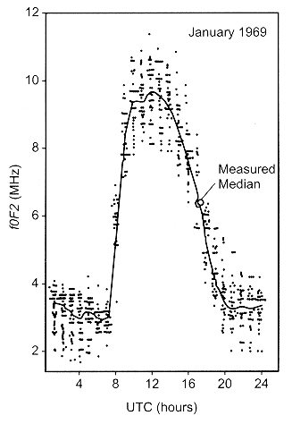
Fig 3 - Ionospheric variability shown by foF2 soundings from Slough, England (after Piggott and Rawer, Note 1).
Fig 3 shows there are departures of foF2 from the monthly median (50%) curve throughout a day. In that regard, observations show that the amount of departure from the median value varies not only with time of day but also with location and season, being the greatest in the middle of winter night. In addition, ionosonde records show that virtual heights h'(f) of reflection for a given frequency f vary with location, sunspot number, whether it is day or night, the season in the temperate zones as well as at low and high latitudes. While one of the IONCAP methods does give statistical values forFOT, MUF and HPF for any path, other statistical variations-say for the critical frequencies and virtual heights-are not given in the methods (1 and 2) of the IONCAP program, which deal with local ionospheric parameters.
Time Variations of Ionospheric Parameters
Another limitation of the IONCAP program is that it only gives predictions at hourly intervals. As a result, nothing is available for shorter periods and the predictions will not show if variations occur on a shorter time scale, say in one of the standard propagation parameters, MUF(3000), the maximum usable frequency for a 3000-km path centered on a given location. That information can be obtained from ionosondes by using shorter sounding intervals; Fig 4 shows soundings taken at five-minute intervals that would apply for the MUF on a 3000-km path centered at Brighton, Colorado, in February, 1981.(2)
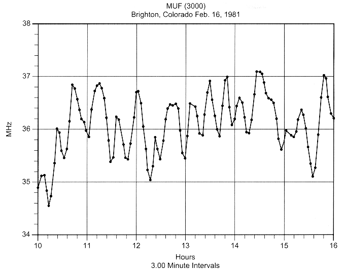
Fig 4 - Temporal variations of MUF(3000) (after Paul, Note 2).
The MUF(3000) variations in Fig 4 show oscillations with the MUF values having periods ranging from 20 to 30 minutes that would not be predicted from the hourly intervals in IONCAP and other prediction programs. Those variations may result from waves propagating through the ionosphere, as suggested by the virtual-height data shown in Fig 5. There, ionosonde data at five-minute intervals, from fixed frequencies near the critical frequency foF2, show wave-like variations with the maxima and minima of virtual heights appearing later at lower frequencies (heights).
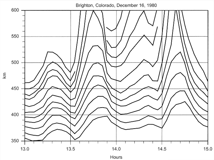
Fig 5 - Virtual height variations at fixed frequencies (after Paul, Note 2).
That particular data set suggests an apparent vertical downward velocity component of about 160 m/s, while the time variations in Fig 4 suggest a wavelength in the range 240 to 360 km. Taken together, the data in Figs 4 and 5 indicates that the main effects of those waves propagating through the F region are a variation of the layer height and-to a lesser degree-of the electron density.
As noted above, programs like IONCAP and the URSI and CCIR databases provide average values of ionospheric variables on an hourly basis. They are more indicative of the slow variations in the ionization levels from solar illumination as the earth rotates beneath it. Accordingly, they reveal none of the ionosphere's more dynamic aspects (which are of internal origin) and how they affect propagation. Since the sounding programs that provided the data on which they are based have long since been terminated, there is little chance to obtain further input to correct the shortcomings noted here.
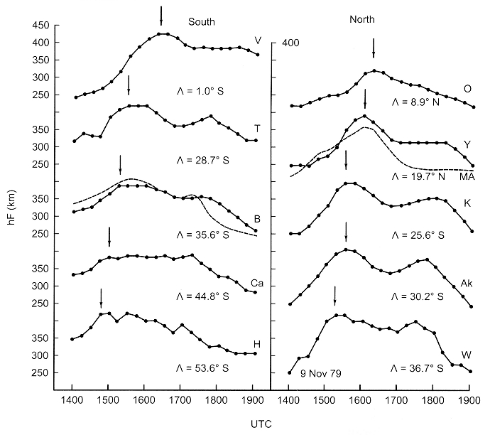
Fig 6 - Variations in the virtual height of the F-region, following the onset of the substorm in the Southern and Northern hemispheres (after Hajkowicz, Note 3).
Atmospheric Gravity Waves
The ionosonde data like those given in Figs 4 and 5 support the hypothesis that F-region variations are caused by atmospheric gravity waves (AGW) with varying amplitudes, which are present all the time. Other data, from more singular events such as auroral substorms, show the presence of AGW at ionospheric heights in different ways, with equator-ward motions from the site of their origin along the auroral zone. Thus, virtual-height recordings in Fig 6 (from 10 ionosondes after the onset of an auroral substorm(3)) show the wave-like propagation of an F-region disturbance that advances from high latitudes in both hemispheres toward the equator. A linear-regression analysis of the first wave crest's advance gives equatorward speeds of 810 m/s and 790 m/s in the southern and northern hemispheres, respectively.
From standard magnetometer and riometer observations at the time of the auroral substorm in Fig 6, the observations were found to be consistent with large-scale traveling ionospheric disturbances (TID) that originated at auroral latitudes in both hemispheres and covered about 60° in longitude. While details of the mechanism at the source are unknown, it seems most likely that the origin of the TID was the AGW, from atmospheric heating with the deposition of energy at auroral heights by the influx of the energetic electrons at the onset of the substorm.
In regard to energy deposition by auroral particles, each pass of the NOAA-12 satellite gives a measure of auroral activity level as well as hemispheric power input (in gigawatts) that is deposited in the hemisphere's auroral zone. Such observations are available and cover the range from quiet (less than 1 GW) to major storm (greater than 500 GW). In addition, an array of sensors on the NOAA POES satellite displays the fluxes going down into the atmosphere, for electrons with greater than 30 keV, 100 keV and 300 keV. The more energetic electrons penetrate down to levels where 160 meter signals are propagated as well as into the lower D region(5) and may affect the level of ionization there, depending on the level of auroral activity.More generally, though, AGW are transverse waves that propagate in the neutral atmosphere and are maintained by gravity and buoyancy, but damped by viscosity. As shown above, they can be seen from the traveling disturbances (TID) they generate in the ionosphere. Sources of AGW5 include not only heating from the precipitation of energetic electrons at auroral altitudes noted above, but also from other large expenditures of energy at lower altitudes. These include tropospheric turbulence, stratospheric winds from weather systems and geological events such as earthquakes and volcanic eruptions.
The large-scale AGW, with periods from 1 to 3 hours and speeds of 500 m/s in the horizontal direction, seem to originate in auroral regions. The medium-scale AGW come up from below the ionosphere, have periods between 20 and 45 minutes and speeds from 80 to 450 m/s. Small-scale AGW, with short periods (2-5 minutes) and speeds the order of 300 m/s, are associated with regions of wind shear and atmospheric turbulence. As shown by the virtual height data in Figs 5 and 6, large-scale AGW affect the height of higher ionospheric regions, thus having a significant effect on the geometrical aspects of HF wave propagation. The same is probably true of the lower F region and the E region, where 160 meter and other MF signals are propagated. Thus, there will be variations in electron density levels at a given geodetic height, as well as density variations from AGW, which produce tilts of the surfaces of constant electron density. Those will contribute to the variability of ionospheric modes through changes in hop length as well as the initiation and termination of ducted signals.
Ionospheric Absorption
Beyond the availability of signals, which is more related to variations of propagation modes and the spatial distribution of ionization than the average electron densities, another matter is ionospheric absorption: a concern at the 160 meter and MF parts of the radio spectrum. Absorption results from collisions between electrons in the lower ionosphere and neutral constituents. For a given frequency, it depends on how the product of the electron density, N, and collision frequency, v, vary with height. In that regard, an estimate of the effective collision frequency as a function of height is given in Fig 7.
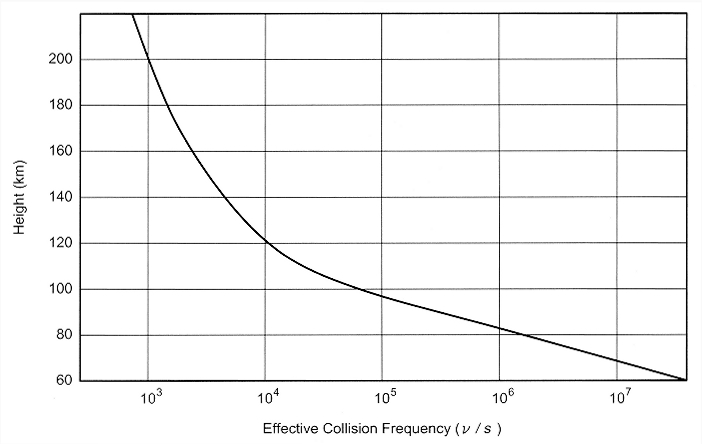
Fig 7 - Effective electron-neutral collision frequency in the lower ionosphere.
While signal strength for a given frequency depends largely on the propagation mode-say, earth-ionosphere hops as compared to ducting additional signal losses result from paths traversing the lower D region between ground reflections. At lower altitudes, Fig 7 shows the collision frequency varies as the neutral particle density and for 160-meter and MF propagation, the lower region is most important since the Nu product is the largest there. In addition, it is the most variable because of changes in the electron density from dusk to dawn, dawn being when signals reach their greatest strength.
The signal loss at a given height depends on the electron density in the lower D region and according to the International Reference Ionosphere (IRI90),(6) that can differ by as much as a factor of two between dusk and dawn. That serves to make the absorption greater at dusk by that factor. The IRI does not deal with details of the ionospheric processes, only the results of many years of ionospheric sounding.
The Role of Negative Ions
Conversely, laboratory data(7) and observations of low-frequency propagation(8) indicate a higher electron density at dusk compared to dawn. The lower electron density around dawn results from electron attachment to molecules, forming negative ions with a high electron affinity. The presence of atmospheric ozone serves to maintain negative-ion attachment until solar UV reaches the D region on rising above the ozone layer (see Note 8). Nothing similar is found at dusk, and the negative ions formed in the D region as the sun sets apparently have lower electron affinities and undergo detachment processes from visible light until in full darkness.
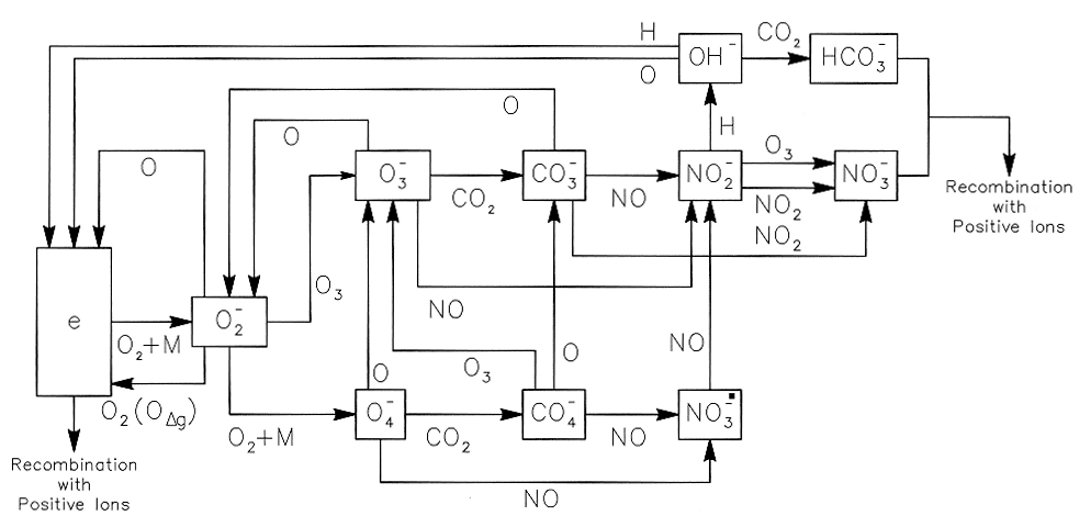
Fig 8 - Schematic diagram of negative-ion reactions (after Reid, Note 7).
Now, current theoretical considerations indicate that the formation of negative ions depends on the series of ionic reactions summarized in Fig 8. There, we can see that it starts with electron attachment to molecular oxygen and then proceeds toward the right of that figure by processes which depend on minor atmospheric constituents. In that regard, for propagation purposes, the left-hand side of the figure can be considered as the start, at sunset. Electrons attach to molecular oxygen and ion reactions then proceeding toward the right-hand side, ultimately giving the final, stable ions in the dawn ionosphere. Close examination of the figure shows the various steps in which ozone (O3), carbon dioxide (CO2), nitric oxide (NO) and hydrogen (H) are involved. The actual availability of those minor constituents depends on vertical and horizontal transport processes in the atmosphere, starting from the photo-dissociation of molecular oxygen, vehicle exhaust, use of nitrogen fertilizer and the water vapor. Thus, in the course of a night, those molecules can combine with the simple negative ions of oxygen after sunset and develop into bicarbonate ions (HCO3-) and nitrate ions (NO3-), which hold their electrons closely. It is possible that progress of ions from left to right in that figure may be subject to bottlenecks caused by a lack of one or more minor constituents. At one time or another, there may be a low density of ozone here or nitricoxide there, at one place or another. All that means that the lower ionosphere, where 160 meter propagation takes place, is not always a uniform regioneither in composition or in ionization during the hours of darkness. Indeed, going from the sunset terminator to the sunrise terminator, slow development of the negative ions that hold electrons closely has consequences for low-frequency and 160 meter propagation.
Thus, negative-ion species mutate from one with a low electron affinity (less than 0.5 eV) at sunset to another with a large electron affinity (greater than 4.5 eV) at sunrise. This means that kinetic detachment of electrons by atomic oxygen at sunset would serve to yield a significant electron population in the D region. Only as atomic oxygen production comes to a halt after sunset would negative ions start to form, albeit slowly, and begin to decrease the electron density in the lower D region. Accordingly, signal absorption on 160 meters would be greater in the hours after dusk than sunrise.
Electron Detachment
There is one bright side to this picture, which is related to the greater electron affinity of negative ions near the sunrise terminator. It requires solar-ultraviolet radiation to photodetach electrons from those negative ions at sunrise. Therefore, the sunrise on the D region with visible radiation is not effective in detaching electrons held by the negative ions. Studies of LF propagation (see Note 8) show that UV detachment is delayed about 15-20 minutes relative to sunrise with visible radiation, as the solar UV must surmount the ozone layer. That gives DXers a bump, as it were: DX signals last a bit longer before catastrophic D-region absorption sets in.
That was the good news; the bad news is that the ozone layer is quite variable in space and time, so one DXer could enjoy the benefit of the ozone delay, while another might not. That is also quite unpredictable, not only because of the variability of the ozone distribution, but also because the ozone layer, being concentrated at a lower altitude than the D region, casts its shadow on the traversal of signals through the D region from a distance of several hundred kilometers away, in the direction of the rising sun. Atmospheric conditions at such distances would be completely unknown to the DXers and in addition, each path would have the sun rising on the D region at a rather different bearing, compounding the matter.
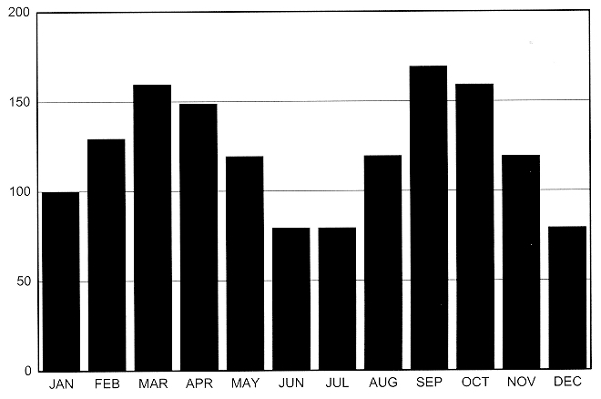
Fig 9 - Monthly distributions of major magnetic storms from 1868 through 1992.
Seasonal Effects
DXing on 160 meters is done primarily in the winter months when there is a greater probability of darkness on paths of interest. Of course, that brings up the question: Are there are any seasonal effects that should be noted, predictable or otherwise? In that regard, long-term magnetic records show that magnetic storming is most probable at the equinoxes and least predictable at the solstices, as shown in Fig 9. That is a statistical summary of magnetic disturbances, a result of observations over many decades. At given time, the situation may from the average because of the current level of solar activity, coronal-mass ejections (CME) and streams of solar wind from coronal holes or flares. So, about the best guidance for 160 meter DXing is to log the indices of magnetic activity as they occur and look for a recurrence of the quiet conditions that go with low indices with the next solar rotation. Nevertheless, sporadic events may still disrupt DXing.
With meteorological factors affecting propagation, features of weather systems may be involved in the winter months. Wind shears and turbulence produce irregularities in the electron distribution up to 90 km in the D region, as noted by Davies(9) concerning the forward scatter of VHF signals. Those irregularities would affect the distribution of ionospheric electrons in the region, one way or another and with all the predictability of weather. Beyond D-region electron-density distributions, there are also effects of minor constituents in that region, which are affected by seasonal variations. In that regard, the negative-ion chemistry shown in Fig 8 is subject to the distribution or availability of minor constituents. Of particular interest are ozone (O3) and nitric oxide (NO), which advance the ion chemistry reactions to the right toward more stable negative ions.
As noted earlier, transport processes play an important role in the distribution of ozone and, day by day, its distribution is quite dynamic. On the average, however, ozone has a seasonal maximum in the spring in the Northern Hemisphere.(10) One type of dynamic event in winter is sudden stratospheric warming, and motions of the atmosphere during those events produce major rearrangements of chemical species such as ozone. In that regard, ozone flows from its site of production at low latitudes to middle and high latitudes, the flow sloping downward toward the pole. That flow is responsible, in part, for the increase in total ozone content at high latitudes.
The seasonal changes in the ozone distribution were quite evident in the LF study (see Note 8), which showed the importance of negative ions in the dawn ionosphere. The changes presumably play a significant role in negative-ion formation in the lower D region between dusk and dawn. The variation of negative ions from dusk to dawn serves to reduce the electron density in the D region. Thus, one can say that any increase in ozone density with a sudden stratospheric warming would decrease ionospheric absorption at night, not increase it.
Nitric oxide (NO) is another minor constituent of the atmosphere that is involved in negative ion formation. There is also a seasonal variation in its formation and circulation, with NO being formed from atomic nitrogen released at E-region altitudes during auroral bombardment.(11) The NO is then carried pole-ward by meridional circulation; as it cools, it descends and the circulation returns it equator-ward. NO has a long lifetime around the dark, winter polar cap. With the return circulation, part of the NO spills out at mid-latitudes and is responsible for the "winter anomaly"(12) in absorption that is found on medium frequencies during daylight. In that case, the NO becomes an additional target for solar UV and when ionized on illumination, serves to increase the electron density in the D region. There is a great deal of folklore about the negative effect of the winter anomaly on DXing in amateur circles. Unfortunately, those who continue to promulgate that idea fail to realize that it is an effect when the ionosphere is illuminated, not during darkness on paths when DXing is done.
Contrary to that negative aspect, circulation of additional NO would add to its role in the formation of negative ions with large electron affinities during time of darkness in the D region. Like the case with ozone, that would serve to reduce the electron density in the lower D region and serve to lessen any absorption rather than increase it.
The ideas dealing with meteorological aspects of 160-meter propagation cannot be related to many observations at the altitudes of interest. Instead, what measurements of the neutral atmosphere that do exist are for lower altitudes: ground-based observations of temperature, pressure and winds, or else satellite views of weather systems from cloud-cover and infrared data. In short, the features of 160-meter propagation where the neutral atmosphere comes into play are essentially unknown to DXers. Consequently, there is little to use in anticipating what propagation would be like. For that matter, even what constitute average conditions are essentially unknown: So the question as to the departure from normal conditions is moot.
At this time, the only method that works reasonably well applies to predictions on paths that go to high latitudes; it involves logging the level of magnetic activity and looking for recurrences. That is based on the effects of long-lived solar streams that sweep by the Earth. It works reasonably well from late in a solar cycle to the rise toward greater solar activity in the next cycle. During the peak of solar activity, magnetic activity is more related to individual solar outbursts-say, coronal mass ejections (CME) and flares. So any propagation planning is strictly short-term in nature, using announcements from the NOAA Websites on the Internet.
Summary
Propagation in the upper HF spectrum results from the ionization of the atmosphere on a global scale by the sun, which is a strong but variable source of radiation. In addition, the slow recombination of electrons and positive ions at high, F-region altitudes contributes to the duration of the ionization, while its distribution is largely controlled by the geomagnetic field, another agent of global dimensions. Those ideas are well understood and propagation resulting from them proves to be quite predictable when bursts of solar and magnetic activity are taken into account.
In contrast to that situation, propagation at the lower Amateur Radio spectrum results from steady but weak sources of ionization: UV in starlight, galactic cosmic rays and solar radiation scattered into the dark hemisphere by the geocorona. The distribution of that ionization near the E region is subject to altitude and density variations from two sources:
- Motions of the neutral atmosphere caused by atmospheric gravity waves
- Vertical and horizontal transport of minor constituents, which play a role in negative ion formation
The principal role of the geomagnetic field at the low end of the spectrum is to provide an efficient propagation mode by means of ducting in the ionization valley that develops just above the E region at night. Of course, magnetoionic theory shows that wave polarization is important there too, and non-reciprocity of paths becomes important because of polarization mismatches between waves and antennas.
Also, as another example, ray-tracing calculations (see Note 4) with the PropLab Pro software show that ducting is more likely on ray paths that are quasi-longitudinal. That is, close to the direction of the geomagnetic field lines, rather than on paths that are quasi-transverse to the field. Thus, signals from the lower magnetic latitudes may be ducted quite efficiently toward higher latitudes, while those in the return direction are more likely to be propagated as lossy earth-ionosphere hops because of the large magnetic dip angle where they originate. Along the same line, there can be large losses in getting waves in and out of the ionosphere, from mismatches in power coupling between antenna polarization and limiting wave polarizations on entrance to and exit from the lower ionosphere. That proves to be particularly important when using vertically polarized antennas for E-W propagation at low latitudes.(13)
Finally, in the HF case, the few parameters available and activity updates on solar-terrestrial conditions generally prove to be sufficient for the purpose ofpropagation predictions. At the low end of the spectrum, other than activity updates, the magnetic indices and satellite measurements of the power input by auroral electrons are about all that are available. They serve only to show when high-latitude paths might be subject to more absorption from auroral ionization, path skewing from that same source of ionization or the precipitation of radiation belt electrons at lower latitudes during magnetic activity.
However, perturbations of the neutral atmosphere from transport processes and atmospheric gravity waves along propagation paths affecting ionization density, heights or path geometry, cannot be predicted or dealt with. There arejust no measurements being made that bear on the questions. In that regard, one is left with the conclusion that meteorological factors make 160 meter propagation even more unpredictable than the weather itself for the lack of observations, especially since not even average conditions are well documented.
Notes
- W. R. Piggott and K. Rawer, URS1 Handbook of lonogram Interpretation and Reduction, Report UAG-50, World Data Center A for Solar-Terrestrial Physics, Boulder, Colorado, 1975.
- A. K. Paul, "Medium Scale Structure of the F Region", Radio Science, Vol 24, No. 3, 1989, p 301.
- L. A. Hajkowicz and R.D. Hunsucker, "A Simultaneous Observation of Large-Scale Periodic TIDS in Both Hemispheres Following an Onset of Auroral Disturbances", Planetary Space Science, Vol 35, No. 6, 1987, p 785.
- R. R. Brown, "Signal Ducting on the 160 Meter Band", Communications Quarterly, Spring 1998, p 65.
- R. D. Hunsucker, "The Sources of Gravity Waves", Nature, Vol 328, No. 6127, 1987, p 204.
- D. Bilitiza, International Reference lonosphere (IRI 90), NSSDC 90-22, National Space Science Data Center, Greenbelt, MID, 1990; nssdc.gsfc.nasa.gov/index.html.
- G. C. Reid, "Ion Chemistry of the D-region", Advances in Atomic and Molecular Physics, Vol 12, (San Diego: Academic Press, 1976).
- R. R. Brown, "Atmospheric Ozone, a Meteorological Factor in Low-Frequency and 160-Meter Propagation", Communications Quarterly, Spring 1999, p 97.
- K. Davies, Ionospheric Radio, (London: Peter Peregrinus Ltd, 1989).
- M. L. Salby, Fundamentals of Atmospheric Physics, (Academic Press, 1996)
- R. R. Garcia, Susan Solomon, Susan K. Avery and G.C. Reid, "Transport of Nitric Oxide and the D-Region Winter Anomaly", Journal of Geophysical Research, Vol 92, 1987, p 977
- E. V. Appleton and W.R. Piggott, "Ionospheric Absorption Measurements during a Sunspot Cycle", Journal of Atmospheric and Terrestrial Physics, Vol. 3, 1954, p 141.
- R. R. Brown, "Demography, DXpeditions and Magneto-Ionic Theory", The DX Magazine, Vol X, No. 2, March/April 1998 , p 44.
References
A. Brekke, Physics of the Upper Polar Atmosphere, (New York: Wiley & Sons, 1997).
R. R. Brown, "Unusual Low-Frequency Signal Propagation at Sunrise", Communications Quarterly, Fall 1998, p 67.
NM7M, bobnm7m@cnw.com