Rob's web

The art of making and measuring LF coils

Home - Techniek - Electronica - Radiotechniek - Radio amateur bladen - QEX - The art of making and measuring LF coils

---

Large, high-quality coils are an importantfactor in working the LF bands successfully. This short note on the specific art describes good quality-factor coils (Q = 600) for 136 kHz.

The "new" band of 136 kHz in Europe and the "lowfer" 160-190 kHz band in the USA are to be considered a good mix between the old fascinating era of Marconi antennas (plus specific grounding topics) and the technologically advanced world of DSP and related high-precision spectrum and noise analysis. Combining modern PC processing capability with very interesting old-style experimentation on big coils and big vertical antennas with capacitive hats, we can obtain unique results (see Ref 4). A very simple transmission circuit to start operation at 136 kHz is shown in Fig 1.

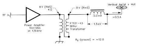
Fig 1 - A simple 136-kHz linear amplifer using a low-cost monolithic IC.

The circuit includes an audio power amplifier commonly used in highquality TV sets: the TDA7265 made by STMicroelectronics.(1) The PC board and heat sink are shown in Fig 2 and complete technical information is available on the Web site (www.st.com).

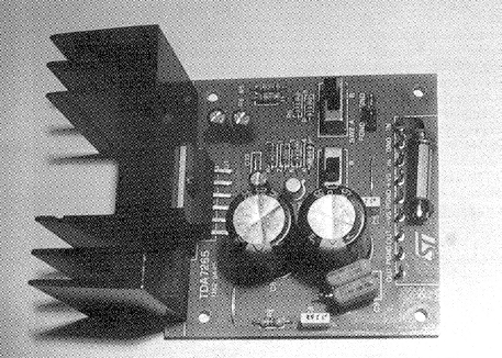
Fig 2 - The ST board designed for 25-W stereo high-quality audio for TV (TDA7265).

The typical output power of the amplifier at audio frequencies is 25 W with 4 Ω speakers; but at 136 kHz, the output power drops to 3-4 W, maximum. This power is more than adequate for LF system tests, generating up to 0.5 A of antenna current.(2) The transformer, T1, is constructed on a standard FT101-43 one-inch toroid core and is used to match the specified 4 Ω load to the 16-20 Ω total resistance of the antenna system (antenna + coil + ground). To check the complete system, a relatively simple antenna is used, with a vertical (Marconi) rod of 7-10 meters isolated from ground using a plastic plate. About 40-50 meters (130-160 feet) of horizontal wires (hat) are connected atop the Marconi antenna to realize a 450 pF total antenna capacity. This establishes a near unity ratio between the top and base currents in the antenna (Fig 3). As you can see from the diagram (from Ref 1), the radiation resistance of our antenna at 136 kHz is very low: about 0.03 Ω. For comparison, the height for a similar antenna at 14 MHz would be 7-10 cm!

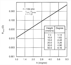
Fig 3 - Radiation resistance versus height of Marconi vertical antennas plus capacity hat.

More complete technical documentation on the big antennas is available in the paper of Ref 1 (Monster Antennas). The ground connection is another big problem at LF, but if you have a country house with a big garden, you don't normally have a ground problem. As is well known, earth is inherently a rather poor conductor, with normal resistivities in the range of 10-300 Ω per meter, and the conductivity of the metal constituting the grounding rod is not very important.

The ground resistance R_G can be pictured as the resistance resulting from a series of equally thick concentric earth shells around the ground rod. With a typical 3-meter rod, half of the resistance is contained within a cylinder of 12-cm radius around the rod (Ref 3). The only way to reduce the ground resistance is with the addition of multiple electrodes. Adding more ground rods reduces the grounding resistance, but the gain is less for each additional rod. That is, the final resistance for many rods is greater than the value obtained by simply dividing the resistance of a single rod by the number of parallel connected rods. A single 3-meter rod of 16 mm diameter driven into soil with 100 Ω/meter average resistivity will have a ground resistance (measured at 50-60 Hz) of 30-50 Ω. Using four parallel rods placed at 10-15 m in a square will give a final LF resistance of 10-15 Ω. At 136 kHz, the inductance of the connecting cables is not important, but we must use a big wire to avoid skineffect resistances. As seen in Table 2 for 424.18 mm Litz wire, we have only a 0.0164 Ω/meter dc resistance (probably less than 0.5 Ω of RF resistance for a 10 meter connection cable).

Table 1 - Wire Table including calculated RAC/ RDC at 136 and 200 kHz

Diameter (mm)	Diameter (mils)	RDC (Ω/m)	RAC/RDC at 136 kHz	RAC/RDC at 200 kHz
0.050	1.97	8.9300	1.000	1.000
0.100	3.94	2.2330	1.000	1.000
0.180	7.09	0.6893	1.001	1.002
0.200	7.98	0.5583	1.002	1.004
0.300	11.80	0.2481	1.011	1.022
0.500	19.70	0.0893	1.075	1.149
0.900	22.86	0.0276	1.507	1.785
1.000	39.40	0.0223	1.650	1.962
2.000	78.80	0.0056	3.060	3.640

Table 2 - Litz-Wire Table for typical Copper Wires

Diameter	Diameter	Litz Wire #	RDC (Ω/m)	RDC Litz (Ω/m)
0.051	2.010	100	8.510	0.0851
0.051	2.010	200	8.510	0.0425
0.051	2.010	600	8.510	0.0142
0.063	2.480	60	0.0031	0.0907
0.127	5.000	50	0.0127	0.0272
0.180	7.090	15	0.6890	0.0459
0.180	7.090	30	0.3445	0.0229
0.180	7.090	42	0.6890	0.0164
0.300	11.810	30	0.2480	0.0083

When using four or more parallel ground connections, the resistance of the wires is not very important. In our tests, two 4 meter deep rods and two 2 meter deep rods were used at a distance from the common ground point (at the base of the Marconi vertical antenna) of 10-15 meters. The measured value of our ground resistance at 136 kHz is R_G = 12-14 Ω. The system's total load resistance seen by the output transformer is:

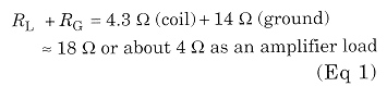
The very poor efficiency of any short vertical Marconi system can be calculated simply using the expression:

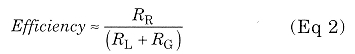
where
R_R = Radiation resistance (see Fig 3)
R_L = Coil resistance
R_G = Ground resistance

The Coils

The load coils used in LF transmitters must have a very high quality factor, Q, or a low equivalent series resistance (for example, R_AC < 5 Ω so as to reduce the transmission losses.

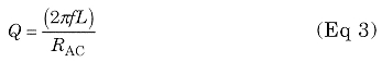
where
f frequency (kHz)
L inductance (mH)
R_AC = LF equivalent series resistance (Ω)
As stated in the introduction, because of the very low antenna efficiency and the relatively high resistance of the Earth (R_G ~ 10 to 15 Ω, see Fig 4), the use of low-Q coils is not practical.

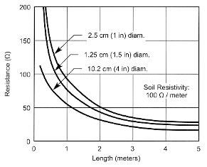
Fig 4 - Ground resistance versus rod length in a typical earth (100 Ω x meter)

The losses that affect the quality factor of LF coils are:

• Skin effect of wires
• Proximity effect between turns of winding
• Lossy dielectric of the distributed capacitance
• Lossy coil form material (such as gray PVC)

In the following, we will consider in more detail both the skin and the proximity effects in the RF windings. Now, we limit our discussion by writing that skin-effect problems are avoided by using Litz wire (which is many thin, insulated wires connected together at the ends). We take this opportunity to remind that, to manufacture some monster antennas, 3.5-inch Litz wire (9 cm diameter!) has been used. The dielectric losses are related to the material used to insulate the conductor-enamel, for instance of the winding. In any case, this kind of loss is very small considering the total tuning capacitance for LF resonance.

During the beginning phase, we tried a gray PVC tube as a form. This tube is often employed in the manufacture of buildings.

Table 3 - High quality coils measured in the LF range

Coil #	Core material	Diameter (mm)	Wire size (mm)	Litz wire (n)	Turns (N)	Coil lenght	D/Len	Wire lenght (m)	L (mH)	RDC (Ω)	136 kHz XL (Ω)	Q	RAC (Ω)	200 kHz XL (Ω)	Q	RAC (Ω)
L01	grey PVC	160	0.90	none	175	176	0.91	88	3.12	2.43	2665	205	13.0	3919	187	21.0
L02	air + wood	160	0.18	30	120	210	0.76	60	1.40	1.38	1196	513	2.33	1758	534	3.29
L03	air + wood	200	0.18	42	157	272	0.73	99	2.70	1.63	2306	507	4.55	3391	435	7.80
L04	air + wood	330	0.90	none	85	87	3.80	88	3.30	2.43	2818	237	11.9	4145	230	18.0
L05	air + wood	330	0.90	none	85	165	2.00	88	2.50	2.43	2135	318	6.71	3140	309	10.16
L06	air + wood	330	0.18	42	94	168	1.96	97	3.00	1.59	2562	597	4.29	3768	541	6.97

This was the worst case we found: Table 3 compares the Q of coil L01 with the other coils wound on wood and air.

The best case used a form of eight wooden dowels connected together by two wooden plates. This core minimizes the mass of material within the solenoid winding. An example of this arrangement is shown in Fig 8A, where the core of coils L03 and L04 (of Table 3) is shown before the wire was wound. To verify the core material's quality, we made a hole in the center of the two wooden plates for the purpose of inserting a big, cylindrical mass of wood. No change in measured Q values was detected while performing this experiment.

To the contrary, a 30% drop of Q is verified when using gray PVC rods. The LF coil-design goal is high performance, with:

• Wires able to sustain high RF currents
• Good insulation
• An inductance value of a few mH

To transmit adequate RF power, we need to produce a load-coil current of a few amperes. This means using a conductor of suitable cross section to carry the 1 to 5 A currents with low RF series resistance. For instance, if we have 3-mH coil in which a current of 1 A flows, the voltage at the coil terminals is about 3000 V (3 mH is +j2563 Ω at 136 kHz and +j3770 Ω at 200 kHz). This is a very dangerous voltage. Moreover, it is necessary to consider the potential difference between two adjacent turns (25 to 40 V with 1 A of current flowing and proportionally higher with increasing current) to set requirements for dielectric strength of the conductor's insulation. The inductance of the coil, for LF purposes, can be calculated using the following equation, considering that it must resonate with the total antenna capacitance (vertical antenna plus top-hat capacity):

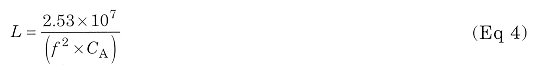
where
L coil inductance (mH)
f frequency (kHz)
CA = vertical antenna + hat capacitance (pF)

At this point, it is necessary to find the number of turns (starting from the inductance computed with Eq 4) and the geometrical dimensions of the coil:

where
N = number of turns of solenoid winding
L = inductance (mH)
d = wire diameter (mm)
k = turns packing factor (greater than 1)
D = coil diameter (mm)

The above formula allows an accuracy of about 1% for a single-layer coil. This was confirmed by the obtained experimental results.

Before calculating the number of turns, N, it is necessary to minimize the proximity effect (see next paragraph). For this purpose, the factor k, which is greater than 1, has been introduced to consider when the distance between two adjacent wires (pitch) is greater than the diameter of the wire, d. The diameter of the coil must be chosen to minimize the wire length in order to minimize the series equivalent resistance: By reducing R_DC, R_AC is also automatically reduced. In Fig 7, we show two graphs that are very useful for coil optimization. In the first graph, we have wire length versus form factor (D/Len); in the second, we have calculated wire length versus coil diameter.

Considering a maximum increase of the conductor length of 5%, with reference to best-case D/Len = 2.5, a maximum change in the coil form factor D/Len from about 1 to 4.8 can be accepted. On the second graph, we can find the coil diameter that we can put into Eq 5 to calculate the number of turns. For instance, considering spacing (pitch) between two adjacent turns of 2 mm, we can use a coil diameter between 260 and 570 mm to obtain a coil with 3 mH of inductance.

Fig 7-Minimum coil wire length versus coil diameter and D/Len; a starting point to realize high-current and high-quality inductors

Fig 7 also shows the value relative to the final coil, L06, to show the optimization performed. The complete characteristics of the other coils are shown in Table 3.

Having chosen the value of coil diameter in the range reported above, the number of turns of the solenoid can be easily calculated. At the end of the theoretical calculations, we go to the practical realization of the load inductor. As already stated, Table 3 shows all the coils tested to verify the optimization also from the practical point of view. L01, L04 and L05 coils have been manufactured using only enameled wire with a 0.9-mm diameter. The first inductor, on a gray PVC support, has the lowest quality factor Q = 205 at 136 kHz and 187 at 200 kHz) because of the bad core material used. The second one has a higher Q (237 at 136 kHz and 230 at 200 kHz), which is related to the better support but affected by the proximity effect due to the closeness between the adjacent wires (k=l). L05 has the highest quality factor of this coil group (318 at 136 kHz and 309 at 200 kHz) due to the increased distance between the subsequent turns (k=2). This last result shows the big influence of the proximity effect on the equivalent series resistance (which we've alrea pointed out) in the LF range.

Remaining coils have been made using Litz wire: L02 with 2x15x0.18 mm, L03 and L06 with 42x0.18 mm wires. The L02 inductor has a very good Q, but it is not useful for our purpose. It has only 1.4 mH of inductance and cannot resonate with the total antenna capacitance, which is estimated to be about 450 pF, considering both the vertical antenna and the top hat.

Fig 8 - A, a simple wood support structure with no LF power loss. At B, the final load inductor (diameter = 33 cm, Q ~ 600 at 136 kHz).

Table 4 - Other intersring coils measured by Bill Bowers. *R_AC=X_L/Q

Coil #	Diameter (mm)	Wire size (mm)	AWG	Litz wires (n)	Turns (N)	Coil lenght (mm)	D/Len	Wire lenght	L (mH)	200 kHz XL (Ω)	Q	RAC* (Ω)
B01	483	1.830	14	1	42	193	2.5	64	1	1256	325	3.86	0.53
B02	483	0.127	36	50	44	241	2.0	67	1	1256	300	4.19	1.82
B03	483	0.127	36	50	40	160	3.0	61	1	1256	400	3.14	1.65
B04	483	0.127	36	50	37	102	4.7	56	1	1256	345	3.64	1.53
B05	483	0.127	36	50	42	193	2.5	64	1	1256	410	3.06	1.73
B06	483	0.051	44	200	42	193	2.5	64	1	1256	430	2.92	2.71
B07	483	0.051	44	600	42	193	2.5	64	1	1256	625	<2.01	0.90

The best coil for our experimental LF transmitter is L06 (Fig 8B); it has a very high Q (597 at 136 kHz and 541 at 200 kHz) and a suitable inductance: 3 mH. For comparison, Table 4 shows some coils realized and measured Bill Bowers (Ref 10). Apart from the reduced value of inductance for these coils (only 1 mH) and according to our experience, we believe that the author did not realize the real importance of the proximity effect with respect to inductance quality factor.

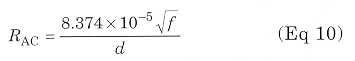
Qs greater than 625 (over the Boonton Q-meter range) related to two factors: the "distributed" turns and big Litz wire with 600 strands. Remember however that obtaining Q of 600 at 3 mH is not so easy as with 1 mH! We think fore that the use of Litz wire having 600 strands of 0.051 mm diameter is an unnecessary complication considering the skin effect. Also see Tables 1 and 2 and remember that R_AC/R_DC = 1.001 (!) with d = 0.18 mm at 136 kHz. At this frequency, the best Litz choice is probably 20 strands of 0.30-mm diameter. Where only direct current flows in a conductor, the resistance has the lowest value and the current density is uniform in the whole cross section of the wire.

where
R_DC = resistance for unit of length (Ω/m)
d = wire diameter (mm)

For alternating current (RF), the current density is not uniform within the conductor cross section and the resistance increases. The current-density change can be explained by considering that the wire is composed of many tubular, concentric conductors. Because each tubular conductor is submitted to the external magnetic field, the inner elements link more magnetic flux than the outer ones. The consequence is an increase in inductance, and so of the reactance, in the part of the wire nearest the longitudinal axis. This is the reason why the alternating current flows mostly in the external surface of the conductor, which can be considered its skin. This effect already begins to be significant at LF (30 to 300 kHz frequency range) when using wires having a diameter that is large (3 - 4 times) compared to the skin depth.

The skin depth is the distance below the surface of the conductor where the current density drops to 1/e (~37%) of its value at the surface. The following relation describes the decrease of current density versus the distance from the wire surface, x (Ref 9):

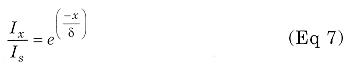
where
I_x = Current at depth x
I_s = Current at wire surface
e = Base of natural logarithms
δ = the skin depth defined by Eq 8

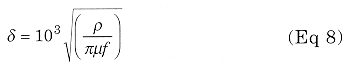
where
p = wire resistivity (~2-meter)
µ = wire material permeability (Henries/meter)
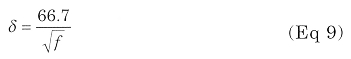
f = frequency (Hz).
Considering a copper wire at 20°C,
ρ = 1.754 x 10-8 Ωm
y = 1.256x 10-6 x µ, H/m; µ_r = 1

A graph of skin depth versus frequency is shown in Fig 6.

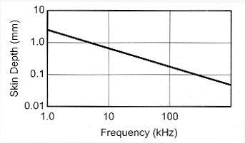
Fig 6 - Skin depth versus frequency in copper-wires. At 136 kHz, the skin depth is 0.18 mm.

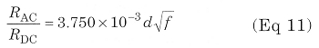
When the diameter of the wire is large compared to the skin depth (at least three times), the useful cross section becomes tubular and the alternating-current resistance can be described approximately by the following equation:

where
R_AC = alternating-current resistance for unit of length (Ω/m)
The consequent ratio R_AC/R_DC, reported below, can be reduced using a tubular conductor with a wide periphery with respect to the cross section. For example, a copper conductor composed of many thin insulated wires can be used, such as Litz wire.

The exact system to calculate the skin effect is reported in Ref 3 of the bibliography.

For the wires involved in our study, Len values are reported in Table 1 both at 136 and 200 kHz. When two or more nearby wires are carrying a current, the current distribution in every conductor is submitted to the magnetic field produced by the adjacent wires. This effect, named proximity effect, increases further the R_AC/R_DC ratio calculated by considering only the skin effect.

The proximity effect is very important in the LF coils, as we verified during the experimental phase of our work. If we consider the L04 and L05 coils (single 0.9-mm enameled wire) of Table 3, the R_AC is reduced simply by increasing the pitch between turns from 1 to 2 mm. The computation of the proximity effect can be performed only on very simple cases that are very far from the single-layer solenoid. At this point, we believe that the better thing to do is to perform the measurements of the quality factor of the coils manufactured by considering all the abovementioned effects together.

Q Measurements

Very few hams own a professional Q meter, and some old equipment (with difficulty) meets the measurement needs of our LF coils: very high quality factor with a few millihenries of inductance.

The first approach is to analyze the possible errors in making the measurement in parallel using a small series resistance (0.5 Ω) to inject RF into the resonant circuit and then measure the voltage at the coil terminals. To measure,coils having a very high Q, it is necessary to consider the quality factor of all the components used in the measurement circuit: RF voltmeter, series resistance, capacitor and interconnections. If, for instance, we have a 3-mH inductance with Q = 600, the parallel resistance of the resonant circuit is greater than 1.5 MΩ (2πfLQ). An RF millivoltmeter with a 10 MΩ input resistance changes the circuit by reducing the measured Q by about 14%.

The other thing that decreases the measured Q is the small series resistance used to introduce the RF signal into the resonating circuit. This effect, together with the RF millivoltmeter effect, reduces the measured Q by about 22%. Nevertheless, all the errors in the inductor quality factor just mentioned are well defined and computable, so the true Q can be calculated.

The last real problem of the parallel measurements is the capacitor loss that it is very difficult to measure because we used an air-variable capacitor. During our experiments, we used capacitors with different dielectric materials; but at the end, we decided to use only an air-variable capacitor for the following reasons:

• Easy tuning
• The very low dissipation factor (0.0001, or a Q=10,000).

These data have been found in the literature and not measured directly. This uncertainty in the quality-factor measurement pushed us to find a better solution. The first idea was to use a toroidal transformer for the RF injection to drastically reduce the series resistance without decreasing the available signal too much. The second idea was to measure the series, rather than parallel, resonance to minimize the loading effects evident before.

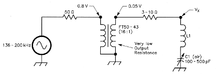
Fig 9 - Circuit for simple and accurate measurments of the quality factor at 136 to 200 kHz.

The proposed circuit is shown in Fig 9. It was used for the measurements in Table 3. The main advantage of this new measurement concept is that it works at very low impedance levels and the R_AC can be evaluated by comparison with the series resistance (R_S = 3 to 10 Ω). When the voltage, V_x, is one half of the voltage at the output of the transformer, the resistance is equal to R_AC and the relevant value (R_S) can be measured by a simple digital ohmmeter, available in any ham shack.

During these kinds of measurements , some shrewdness must be used to prevent possible mistakes. It's important to verify that the coil under test and its magnetic field are far from metallic surfaces and lossy materials (such as a wooden table) so that any such materials do not intercept the fields. Coils having such big dimensions compared with those used in traditional radio applications, become loop antennas. So the measurements must be repeated, putting the winding in different positions and orientations to avoid possible errors.

Another consideration during the measurements is the distances among interconnection wires. They must be so far apart, in spite of the relatively low frequency involved, that they do not affect the result of the test. Considering all these error sources, a possible suggestion is to find a reference inductor to verify the quality of the measurements performed. For this purpose, we used a shielded coil, manufactured by Boonton company and used in Q tests, having the following characteristics: L = 2.5 mH, Q = 170. In Fig 5, this last (relatively small) coil is visible on top right together with the group of inductors realized in our LF operation.

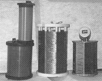
Fig 5 - A group of 136-kHz big coils realized for high quality factor (Q).

Notes

1. STMicroelectronics, 1000 E Bell Rd, Phoenix, AZ 85022; tel 602 485 6100, fax 602 485 6102; us.st.com.
2. A VLF band already exists in the US, but it's not an Amateur Radio allocation yet. A lot of "lowfer" (Low Frequency Experimental Radio) activity occurs in the 160 to 190-kHz region-the so called 1750 meter band, authorized under Part 15 of the FCC regulations. Right now, you don't need a license to operate on 1750 meters, but there are severe legal restrictions on what you can put on the air there. For starters, you can't run more than 1 W input to the transmitter's final stage, and the entire length of the transmission line and antenna combined cannot exceed 15 meters (approximately 50 feet). That's not much antenna for a band where a half-wavelength antenna would be more than one-half mile long! Hams that operate on 1750 meters sometimes use just their call sign suffix as an ID.

References

1. W. J. Byron, W7DHD, "The Monster Antennas", Communications Quarterly, Spring 1996, pp 5-24.
2. W. J. Byron, W7DHD, "A Word About Short Verticals", Communications Quarterly, Fall 1998, pp 4-6.
3. M. Mardiguian, Grounding and Bonding, Vol 2, (Gainesville, Virginia: Interference Control Technologies, 1995) p 2.43.
4. P. Dodd, G3LDO, The LF Experimenter's Source Book, 2nd Edition, (Potters Bar, Hertfordshire, England: RSGB, 1998).
5. P. Dodd, G3LDO, "Getting Started on 136 kHz", RadComm (RSGB), March 1988,
6. D. Curry, Basic 1750 m Transmitting Antenna.
7. Reference Data for Engineers, 7th Edition, (New York: H. W. Sams & Co, 1989), p 6.4.
8. The 1990 ARRL Handbook (Newington, Connecticut: ARRIL, 1989).
9. F. E. Terman, Radio Engineer's Handbook, (New York: McGraw-Hill 1958).
10. B. Bowers, "Low Frequency Coil 'Q'", The Lowdown, Feb 1996. The Lowdown is the monthly newsletter of the Longwave Club of America (LWCA), 45 Wildflower Rd, Levittown; PA 19057, USA.
11. I.R. Sinclair, Newnes Audio and Hi-Fi Handbook, 2nd Edition, (Oxford: Butterworth-Heinemann, 1993), pp 748-752
12. M. Morando, I1MMR, "TX da 10 W a 137 kHz", Radio Rivista (Journal of the Associazione Radioamatori Italiani, Milan, Italy), Sep 1998, pp 52-53.

IW2ACD
IK2WAQ