Improved dynamic range testing
Dynamic range is an important measure of transceiver performance. Learn to avoid the piffialls of measuing it and reap a reward in accuracy.
Dynamic-range testing of transmitters and receivers is increasingly important in view of today's crowded bands. That is evidently true for commercial services, the military and Amateur Radio alike. Recently, I became more aware of certain factors in play during such testing that tend to significantly degrade the accuracy of the results. Let me explain what I discovered and put forth some suggestions for improvement.
What is Dynamic Range?
Dynamic range may be broadly defined as the ratio of the smallest usable signal to the largest tolerable signal. That definition applies as well to transmitters as it does to receivers, but I shall begin my discussion with receivers, since they usually must exhibit larger dynamic ranges than must transmitters.
Noise should determine the lower limit of a receiver's dynamic range. That lower limit may be defined by the signal-to-noise ratio (SNR) of a desired signal at its output. By the accepted standard, the lower limit occurs when a desired signal, modulated by a single sinusoid or tone, has SNR = 0 dB. Then, signal power equals noise power. That power level is called the noise floor. It has also been called minimum discernable signal (MDS),(1) but we are trying to get away from that term because it implies something about individual perception. Many operators and automated systems can discern signals below the noise floor (SNR < 0 dB).
Either noise or distortion may determine the upper limit of receiver dynamic range. When upper-limit measurements are noise-limited, it is often because of so-called reciprocal mixing, wherein noise sidebands on a local oscillator mix with out-of-band interference to produce in-band noise. When upper-limit measurements are distortion-limited, several interrelated mechanisms may be to blame. I leave out any discussion of strong in-band signals here and focus on interference outside the receiver's passband.
Second-order intermodulation distortion (IMD2) occurs when two un desired signals combine nonlinearly to produce their sum and difference frequencies. IMD2 happens when receiver components behave according to a square law. When the level of the two undesired signals is increased simultaneously by 1 dB, IMD2 increases by 2 dB. Third-order IMD (IMD3) occurs when receiver components behave according to a cube law. For every 1 dB of increase in the two offending signals, IMD3 increases by 3 dB. It might seem funny, but receivers can exhibit both square-law and cube-law behavior at the same time.
One quantification of IMD is called intercept point (IP): the power level at which IMD product strengths allegedly rise to match those of each interfering signal. See Fig 1. In modern receivers, IPs may by quite high. It is not unusual to see receivers with third-order intercept points (IP3s) of +30 dBm (1 W) and second-order intercept points (IP2s) of +80 dBm (100 kW). IPs form an excellent basis for comparison of receiver distortion performance. They usually cannot be measured directly at those power levels but must be extrapolated from lower-level measurements.
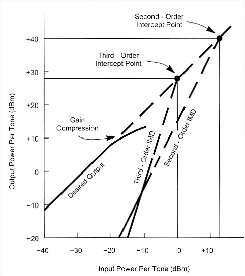
Fig 1 - Showing where fundamental receiver response and IMD intercept.
To do that, one makes the assumption that IMD products behave according to either a square law or a cube law. One injects interfering signals of sufficient amplitudes to produce measurable in-band IMD products and compares power levels. IMD dynamic range (IMD DR) is the ratio of the level of one of two equal-power, off-channel signals producing some inband power, P, equal to the noise floor, to that of a single, in-band signal producing that same power, P.
Sometimes, receiver IMD responses deviate significantly from the straight lines that square-law or cube-law behavior predict. Nonetheless, one generally accepted way to calculate intercept points is to take the noise floor plus twice the IMD2 dynamic range for IP2 and noise floor plus 1.5 times the IMD3 dynamic range for IP3. In a receiver with a classic response, this yields IPs precisely. A more generic formula can be used for any two points along the two lines in Fig 1, without knowing where on the lines the points actually fall. For IP2, the equation is:
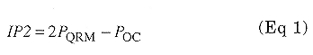
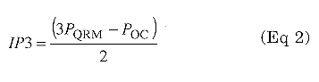
where PQRM is the level of one of the two off-channel signals causing the IMD and POC is the level of an onchannel signal producing an identical output power from the receiver. For IP3, the equation is:
On small-signal measurements and the nature of noise
The chief enemy of small signals is noise. Noise is generated in receivers by the random motion of atomic particles inside circuit elements. A famous paper published in 1905 quantifies it.(2) Physical law states that available noise power is directly proportional to the temperature (in Kelvins) of the thing generating the noise. Noise from a signal source (a test generator) is also delivered to a receiver and it may be significant. That is likely when receiver noise figures are low-less than 6 dB or so. Such noise must be distinguished from receiver-added noise during testing.
A signal delivered from a source to a receiver has a certain SNR in the bandwidth of interest. A receiver's job is to preserve that SNR as best it can. All physical circuits add some noise, though. Under controlled conditions, the ratio of a receiver's output SNR to its input SNR is called its noise factor. When expressed in decibels, the ratio is called the noise figure. To make noise-figure specifications complete, a temperature must be included. Usually, "room temperature" (290 K) is assumed.
I mentioned that noise in signal sources propagates directly to a receiver output. Since noise powers add, noise from signal generators may skew measurements when the noise figure of the thing being measured is low. So the effective source impedance of the noise source must be known during noise-floor measurements. In actual operation, though, low receiver noise figures are not always necessary. A strong, noisy signal on 80 meters, say, would not have its SNR degraded much by a receiver having a noise figure as high as even 20 dB.
Noise may be defined as the output of a randomly driven process. It can be understood by taking a large-scale view of the world. Given the large number of very small particles in the universe and the variety of forces at work on them, it is perhaps no surprise that seemingly random events occur. Some say that given the starting conditions and the laws of basic forces, the state of the universe at any time may be determined from its past state. Others have shown that presumption to break down at very small scales. Such small-scale breakdowns have a way of making themselves evident at much larger scales.
In many ways, we find now that the universe tends to go from a more-or-derly state to a less-orderly state.(3) That situation seems inextricably linked to the passage of time.(4) So many pseudo-random events have occurred since the start of time that the electrical noise we experience may be characterized as truly random.
In a receiver circuit, a noise voltage may take on almost any value. Over relatively short time frames, though, it has some peak amplitude, A, and a peak-to-peak amplitude of 2A. The average value of that noise voltage is zero because it is just as likely to be positive as negative. It is also equally likely to be small as large. One may use these facts to compute the average and RMS power of noise.
Over short time frames, a small leap reveals that the average absolute value of noise having peak amplitude A is A/2. We can prove that by integrating the noise voltage over the range of possible values and dividing by the range:
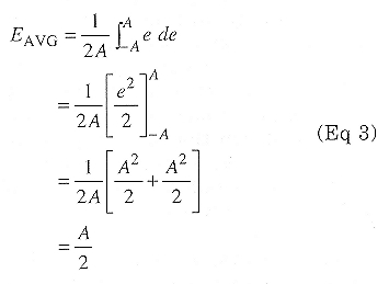
The average power is therefore proportional to the square of that, or A2/4. The peak-to-average ratio of noise is thus about 6 dB over the short haul. To find the RMS value of noise-or any function-take the average (mean) of the square of the function (its mean square), then take the square root of that. For noise, this yields:
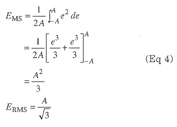
RMS noise power is one-third of its peak power. Compare this with a sine wave, whose RMS power is one-half of its peak power, or with a square wave, whose RMS power is equal to its peak power.
The exercise above is important because it reveals a pitfall that often arises when measuring sensitivities of receivers. A common procedure is to connect an ac voltmeter to a receiver loudspeaker and, in the absence of input signals, set the volume control so that the meter reads 0 dB. A desired signal, usually a single tone, is then injected into the receiver until the meter rises by some amount, often 3 dB or 10 dB, depending on the type of measurement. Normally, 3 dB would be used for a noise-floor measurement.
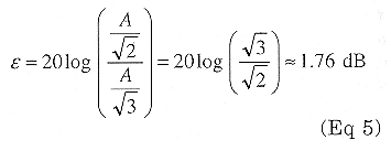
If the ac voltmeter were a peak-reading type calibrated as RMS, it would indicate A/1.41 when the noise alone were present. The real RMS value of the noise is A/1.73, so the error would be:
If the ac voltmeter were an averagereading type, the error would be:
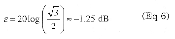
In the first case, the SNR looks worse than it should, while in the second case, it looks better than it should.
A true RMS-reading voltmeter must be used to get accurate results using the voltmeter method. The presence of noise in a 10- or 12-dB SNR sine-wave signal is not enough to produce a significant error in the reading when the voltmeter is calibrated as RMS.
To compute a receiver's noise figure from its noise floor, bandwidth must be precisely known. Noise-floor measurements made with filters having undefined bandwidths and responses do not constitute a good basis for comparison. One receiver's 500-Hz filter might be closer to 350 Hz and another closer to 700 Hz, producing up to a 3-dB difference in noise-floor power even if their noise figures were the same. Passband ripple and stop-band response (shape factor) may throw results off by several more decibels. My first suggestion, therefore, is that noise figures form a more useful basis for comparison of receiver sensitivities than measurements of noise-floor power.
To find a particular receiver's noise figure, its effective bandwidth must be determined. Effective bandwidth is asy to find for filters having flat passbands and low shape factors. It may be computed for any filter by integrating its normalized response over frequency:
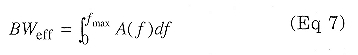
where A(f) is the filter's amplitude response at frequency f. For this computation, the largest value of A(f) found is defined as unity and all other values are normalized to that passband peak. Tones used to measure noise-floor power must be at or near the passband peak. Noise figure may then be computed by finding the difference between the theoretical noise floor of a perfect receiver (NF = 0 dB) and the measured noise floor. In a 500-Hz bandwidth, the theoretical limit is about -147 dBm at room temperature. Noise figure is the true measure of a receiver's noise performance as it provides bandwidth-independent information.
Alternatively, a calibrated broadband noise source may be considered instead of a single tone during noisefloor testing. Theoretically, a receiver's frequency response is then irrelevant because the test signal has energy at all frequencies, but this method has its own pitfalls. It does not account for the effects of poor opposite-sideband rejection and spurious responses of a receiver. A unit with poor oppositesideband rejection, for example, might yield erroneous noise figures because additional energy would appear in the passband that was caused by energy outside that passband.
On the other hand, one can readily measure a receiver having good levels of spurious rejection and opposite-sideband suppression with this method. When the effective source resistance of the noise source is accurately known, a receiver noise figure may be found by comparing its output power with and without the external noise source. Because of its bandwidth independence, many RF designers consider this method the best way to go.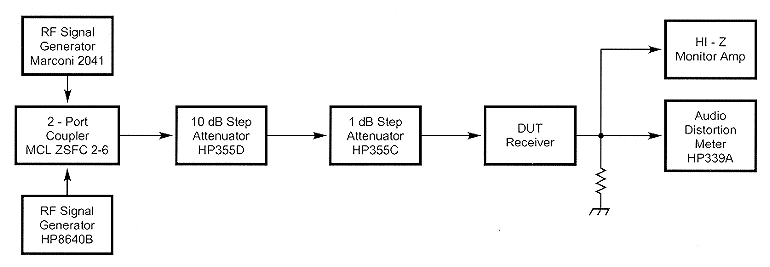
Fig 2 - A typical receiver IMD test setup.
IMD measurements
Receiver IMD measurements involving large, off-channel signals are difficult to perform accurately. One reason for that involves trouble in generating a clean two-tone signal for application to the receiver under test.
A typical test setup for receiver IMD is shown in Fig 2. Two signal generators are combined in a hybrid combiner. The output of the combiner is fed into the receiver via an attenuator. Some isolation between the generators is achieved exclusive of the combiner because typical laboratory generators use internal attenuators to set heir output levels. The external atenuator is strictly necessary because the combiner must be operated into its designed load:impedance to get additional isolation. The hybrid combiner achieves a certain isolation level between generators' outputs when its load impedance is right. In typical combiners, that is no better than about 35 dB. Some energy from each generator appears at the.other and nonlinearity in generator output stages generates IMD in the test signal.
When the combiner output is not correctly terminated, some energy from the combined output signal is reflected back toward both generators. The attenuator in Fig 2 must therefore provide a good termination, equal to the characteristic impedance of the system-usually 50 Ω. For example, were the termination impedance at the combiner output 60 + j0 Ω, the SWR would be 1.2:1 and the reflection coefficient, ρ, would be about 0.10. The isolation between signal generators would be degraded to a value equal to twice the combiner 3-dB insertion loss minus 20 log(0.10) or roughly 6 + 20 = 26 dB.
Sometimes, 35 or even 50 dB of isolation is insufficient to prevent IMD in generator output stages. Some laboratory generators do fine at lesser isolations, but any doubt may be easily overcome during IMD2 testing because the frequencies of the two generators are so far apart. For example, two signals at 6 and 8 MHz may be combined to test for IMD2 at the sum frequency of 14 MHz. It is reasonably simple to employ a low-pass filter at the 6-MHz generator and a high-pass at the 8-MHz generator to increase isolation. Such filtering is generally impractical, though, when two signals 20 or even 5 kHz apart must be used to test IMD3 in receivers. Crystal filters have been used, but even crystal manufacturers have a tough time characterizing the IMD response of quartz, especially at signal powers near 0 dBm. In addition, crystal filters are good for only one set of frequencies. It is better to start with a combiner having very high port isolation.
I have recently discovered how to build broadband combiners exhibiting isolation several orders of magnitude greater than that of ordinary combiners. That is, isolation is typically 65 dB instead of 35 dB. I have measured isolation as high as 90 dB at 200 MHz. Insertion loss is about 6 dB instead of the normal 3 dB, but the net gain in isolation is still quite worthwhile. The ARRL Lab is currently evaluating one of my prototypes.
During receiver IMD testing, a reference power level is chosen. That may be at the noise floor or it may be much higher than that. It should not matter: The idea is to find a point on the line representing the square- or cube-law response of the receiver in the presence of two, equal-level interfering tones. A reference power level much higher than the noise floor is good because it avoids difficulties in measuring noise powers. Noise is constantly changing and as the ARRL Handbook rightly points out,(5) picking a reference level well above the noise floor makes life easier.
Having selected a reference power level, a single, on-channel signal is applied and some measure of receiver response is noted. That can be an indication on the S meter, such as S-5, or an another absolute measure of the receiver's output power. (A measurement that distinguishes the level of the IMD product from the noise is preferred over a broadband measurement. More on this below.) Then the on-channel signal is removed and a clean, off-channel two-tone interfering signal is applied. The levels of the two tones are simultaneously increased until the same S-5 indication is attained. IP and IMD DR are then computed and recorded. This procedure applies equally well to secondorder and third-order tests.(6) The results of tests must produce noise-floor, IMD DR and IP numbers that agree. In other words, IP2 must equal twice the IMD2 DR plus noise floor, and IP3 must equal 1.5 times the IMD3 DR plus noise floor. Published numbers should be accompanied by an estimated margin of error. When the numbers do not correlate within the margin of error, something is wrong.
Take that with a grain of salt, because quite often receivers that are supposed to behave according to perfect square or cube laws act differently in the presence of signals at various levels. Were one to inject signals equal to the calculated IP3 of a receiver, for example, one might find that the real IP3 is much different-or one might "toast" the receiver!
My second suggestion is that as many reference power levels be used in IMD DR testing as are necessary to determine the slope of the IMD line. ARRL Lab Supervisor Ed Hare, W1RFI, demonstrates the need for that nicely in his sidebar "What is the 'Real' Intercept Point?" From the receivers he has measured, note that the calculated IPs strongly depend on the reference levels used. Errors of 10 dB or more are easy to get when taking only one set of points on the response curves. That has unfortunately engendered considerable doubt about accuracy in many instances. While receivers don't always follow square or cube laws exactly, the assumption must be made that they do when finding IPs and some fit to a straight-line response must be sought.Effects of Phase Noise
In the May/June 2002 QEX,(7) Peter Chadwick, G3RZP, took on the task of deciding how much dynamic range HF receivers need. He made some measurements of actual received signal strengths and based his conclusions on those. He found that quite often, phase noise causes reciprocal mixing that masks the IMD performance of receivers.
Phase noise is the unwanted phase modulation of frequency-control elements in a receiver. Especially during IMD3 testing, phase noise may limit one's ability to measure dynamic range. That is because the interfering signals are close enough to one's passband to cause significant reciprocal mixing. In fact, the effect may prevent one from actually measuring the IMD DR of the receiver under test in the usual way. It is an undesirable situation, but it is what led Peter to define phase-noise dynamic range. Phase noise also comes into play prominently during measurement of so-called blocking dynamic range. That measurement is designed to indicate the ability of a receiver to accommodate a single strong, off-channel signal while receiving a weak, on-channel signal. In older rigs, a strong adjacent-channel signal often reduced the output level of the on-channel signal. There could have been several reasons for that, including saturation of some stage or actuation of analog AGC. Modern rigs typically run into the reciprocal-mixing problem before other blocking effects rear their heads, though. Reciprocal mixing generally causes receiver output power to increase, rather than decrease, because of noise mixed into the passband.
Getting back to the case of noise-limited IMD measurements, we are stuck with having to decide how to pick IMD products out of reciprocal-mixing noise. It is not okay to just guess at the IP. I have found an audio spectrum analyzer very useful in digging IMD products out of the noise. The resolution bandwidth of the analyzer may be reduced until a discrete IMD product stands out. So, rather than using a voltmeter to measure receiver output power, a spectrum analyzer is a good tool for measuring the power of a single IMD product alone. When performance is limited by phase noise in every test of interest, though, IMD DR loses much of its relevance.
Transmitters have dynamic range, too
The concept of intercept point applies equally well to transmitters. The chief difference from receivers is that for transmitters, output IP is specified instead of input IP. If an SSB transmitter had lMD3 levels 30 dB below one of two tones at 100 W each, then its output IP3 would be 30 / 2 = 15 dB greater than 100 W, or 15 + 50 = 65 dBm. Such a figure may be used to compare transmitters much as it is to compare receivers, although that is not often done. It is more sensible to talk about a transmitter's maximum output power at some level of IMD.
Tim Pettis, KL7WE, discovered a unique way of combining (with good isolation) the outputs of two transmitters to produce an IMD-free test signal for driving high-power amplifiers during IMD testing.(8) It uses Six 1/4 lengths of coax in two rings. It is a narrow-band solution, so a separate fixture must be constructed for each frequency range tested. Like other combiners, it is sensitive to termination impedance, but it includes a way to adjust isolation for various loads.
Hum and noise measurements are normal parts of transmitter testing. The dynamic range of a transmitter may also be defined in terms of the maximum signal-to-noise- and-distortion (SINAD) ratio it produces.
What is the "Real" Intercept Point?
Fig 1 shows how the relationship between a receiver's on-channel response and third-order intermodulation response can be summarized into a single number-the third-order intercept point (IP3). As seen on the graph, this is the point where the first-order and third-order response lines intersect. The intercept point can be a good way to easily compare one receiver with another. If the response of a receiver perfectly matches the curves shown, the intercept point can be calculated using any two points at the same receiver output level. One would get the same IP3 using measurements made at S9 as one would with measurements made at the noise floor.
Unfortunately, for test and design engineers, real-world receivers do not know that they must follow this theoretical response. In many caees, receivers perform just a little bit differently than expected. This can make the real intercept point of a receiver subject to the judgement of the person looking at the real response curves and trying to decide just what the IP3 of a receiver really is.
The ARRL Lab grabbed a few radios from W1AW and did some IP3 testing. (How many hams would love to be able do that?) The results are shown in Figs A through C. One of the radios behaved pretty close to the theoretical response, but the other two don't really seem to know that their responses are supposed to be straight lines.
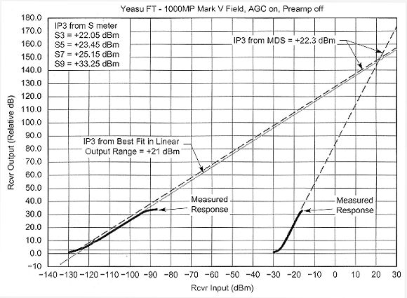
Fig A - The Yaesu FT-1000MP Mark V Field measured in the Lab for this sidebar shows a response that is pretty close to theoretical.
Fig A shows the measured response of a Yaesu FT-1000MP Mark V Field. In this case, the receiver response is, pretty close to what theory predicts. The first-order response (on-channel) increases by 1 dB for every 1 dB of increase in signal, at least up until receiver AGC levels the receiver output. The third-order intermodulation response appears at much higher levels of off-channel signals, and once it appears, the receiver output increases 3 dB for every 1 dB of input level. If one makes measurements of the input levels at any point, one gets approximately the same IP3. Because these are all relative measurements, the receiver S-meter can be used as an indicator of relative receiver output. The inset box in the graph shows the IP3 calculated using various S-meter readings. At S9, the deviation from theoretical has pushed the IP3 up quite a bit. The receiver AGC may be responding to the very strong off-channel signals 20 kHz away.
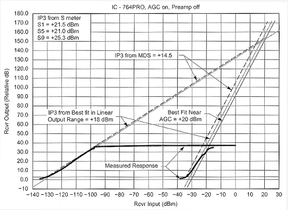
Fig B - The third-order response of the lcom IC-746PRO measured in the ARRL Lab shows less than 3:1 output-vs-input ratio.
Fig B shows a less-classic receiver response-that of the IC-746PRO. In this case, the on-channel response is classic, but the third-order response increases by less than 3 dB for every 1 dB of receiver input. In this case, if one calculates IP3 using measurements made at the noise floor, one will get a lower number than that obtained by using IMID measurements made at stronger signal levels. I speculate that the two signals, spaced at 20 kHz and 40 kHz from the desired signal, may not be at the same level inside the receiver at the point where the intermodulation is occurring.
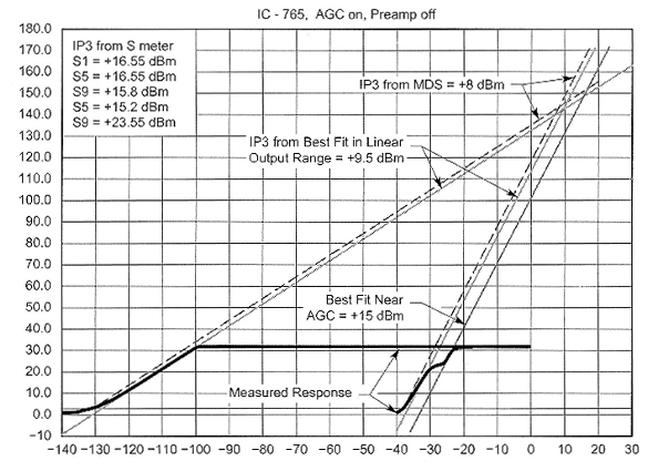
Fig C - What is the "real" intercept point of this Icom IC-765?
The differences in receiver responses have little to do with today's technology. Fig C shows the measured response of the IC-765 we borrowed from W1INF, the ARRL HQ club station. Its third-order response shows a little "burble" within a few decibels of where receiver AGC would become active. In this case, the calculated IP3 is much higher for stronger input levels than it is for measurements made at the noise floor.
As an important aside, none of these deviations from theoretical indicates a receiver problem. They are just artifacts of how very strong signals sometimes behave inside of complex receivers.
In the case of the receivers shown above, what is the "true" intercept point of each receiver? There really is no true number, but one could rightfully argue that one made by using a "best fit" of the theoretical lines against the actual curves best represents the receiver's true IP3. That sounds good in principle, but in practice, doing the tests for these sidebars took considerable time. QST readers want to see Product Reviews as soon as possible, and the ARRL Lab can't take the time to do much extra testing for radios being reviewed. Measurements made at the noise floor are difficult to make, and the influence of the measured noise on an IP3 calculation made from receiver responses at the noise floor is not a very accurate way to make measurements. Even more important, in almost all "real-world" use, the ambient noise level when an antenna is connected to receiver is probably 10 or 20 dB higher than the receiver input noise. In addition, if an intermodulation product is only a few decibels above the noise, it is not going to have as much impact on listening as would one at a higher level. For that reason, the ARRL Lab has used an S5 receiver output level as the point at which IP3 calculations are made since the mid 1990s. This probably represents a reasonable strong signal that is apt to be encountered in the real world. Although this is not quite as accurate as a best-fit calculation, as can be seen from the graphs, an S5 calculated IP3 is reasonably close to the "real" IP3 of the radios tested.-Ed Hare, W1RF1, ARRL Lab Supervisor.
Conclusion
I hope my suggestions help you perform improved dynamic-range testing. Careful methods, good instrumentation and a little persistence lead to accurate and repeatable results. Many heartfelt thanks to Leif Asbrink, SM5BSZ, for getting me going on this topic and for discussing it with me in such a rational manner. He deserves most of the credit for the ideas I present. Thanks also to Ed Hare, W1RFI; Mike Tracy, KC1SX; and Zack Lau, W1VT, for their valuable input and kind assistance.
Notes
- M. Tracy, KC1 SX, ARRL Test Procedures Manual, ARRL, Rev G, Jan 2002. ARRL members may download the manual at www.arrl.org/mem bers-only/prod rev/testproc.pdf.
- 1905 was a good year for Albert Einstein. Along with his papers explaining the photoelectric effect and special relativity came "On the Motion Required by the Molecular Kinetic Theory of Heat of Small Particles Suspended in a Stationary Liquid", Annalen der Physik, 1905.
- T. Ferris, Ed., The World Treasury of Physics, Astronomy and Mathematics (New York: Little, Brown and Co, 1991).
- R. Feynman, Six Not-So-Easy Pieces (Reading, Massachusetts: Addison-Wesley, 1997).
- D. Reed, KD1CW, Ed., The 2001 ARRL Handbook (Newington, Connecticut: ARRL, 2001), p 15.20.
- ARRL Handbook, pp 17.5-17.6.
- P. Chadwick, G3RZP, "HF Receiver Dynamic Range: How Much Do We Need?" QEX, May/June 2002, pp 36-41.
- T. Pettis, "Hy-Brid Hi-Power", Proceedings of the 1998 Central States VHF Conference, ARRL Order #6915.
KF6DX