Fundamental beam patterns
Simplified plotting of antenna characteristics.
Here is a story designed to take a little of the black magic out of how antenna patterns are obtained. By following the principles set forth, anyone can see how some of our common types of arrays "get that way" and what can be expected from them in the way of directivity, and you don't have to be a super-mathematician or slide-rule pusher to figure them out.
Amateurs are becoming increasingly aware of the importance of taking advantage of the directional characteristics of even a simple half-wave antenna, particularly at the higher frequencies, but many may feel that the plotting of directional patterns of common combinations of half-wave elements is too complicated for the average operator. It is the purpose of this story to show that the technique is well within the reach of any interested ham with some paper and a pencil.
Basic patterns
A short review of first principles is in order, for background purposes. It will be recalled that the free-space pattern of a half-wave antenna is a figure-8 pattern revolved about the antenna, and that this pattern is modified by the orientation (horizontal or vertical) of the antenna and its height above ground. Thus the pattern of any half-wave antenna is obtained by multiplying the figure-8 pattern by the ground-reflection factor for the particular height above ground. This subject is elaborated in Chapter Three of The ARRL Antenna Book.(1) The maximum lobe (or lobes) may be at any vertical angle, depending on how many wavelengths or fractions thereof that the antenna is mounted above ground, and it should be kept in mind that all of the patterns to be described are modified in exactly the same manner.
Studying the patterns obtained for a half-wave antenna immediately shows that at some heights above ground there is considerable radiation upward at undesired angles, undesirable because low-angle radiation is the most useful at the higher frequencies. The radiation at undesired angles represents lost power, or at least power that could be utilized to improve the signal strength in a desired direction. This power can be directed to some extent by selecting the proper height above ground, and to a greater extent by combining antenna elements in an "array" and feeding them with currents of correct phasing and amplitude so that the radiation from the individual elements adds in the desired direction and cancels in the undesired directions. In a parasitic array this is done by choosing an optimum spacing, usually between 0.1 and 0.2 wavelength, and tuning the parasitic elements until the correct induced currents flow on the reflectors and directors. The elements are combined in such a way that the radiation from the driven element and the reradiations from the parasitic elements add in the desired direction.
In arrays where all of the elements are driven, there are three basic arrangements that are normally used: collinear, broadside and end-fire, as shown in Fig. 1. The elements can of course be grouped in more complex designs than those shown, to obtain more gain and sharper patterns, but these arrays can always be broken down into a combination of the basic types; e.g., one might have an array of two broadside sections arranged and excited to give end-fire operation through the two broadside sections, and so on. Also, one could consider a broadside array of four elements as a broadside arrangement of two broadside arrays or a collinear array of four elements as a collinear arrangement of two collinear arrays.
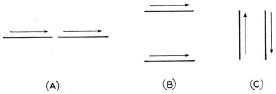
Fig. 1. The three basic types of driven arrays.
The collinear (A) has the axis of each element in the same line and the elements are excited in phase. The maximum radiation is at right angles to the common axis.
The broadside array (B) uses elements in the same plane, spaced from ¼ to 1 wavelength, and the elements are excited in phase. The maximum radiation is perpendicular to the plane of the elements.
The end-fire array (C) uses elements in the same plane, spaced from 1/10 to 5/8 wavelength, and the elements are excited out of phase. The maximum radiation is in the plane of the elements and at right angles to them.
Combining the patterns
In order to compute the beam patterns of arrays that are composed of vertical or horizontal half-wave elements, it is only necessary to multiply the fundamental pattern of the horizontal or vertical element of which the array is composed by the pattern of the group. Table 1 gives the group patterns for vertical elements for the following popular conditions: (A) in phase, half-wave spacing (broadside), (B) 180° out of phase, half-wave spacing (end-fire), (C) 180° out of phase, close spacing (end-fire), and (D) 90° out of phase, spaced quarter wavelength (unidirectional end-fire). The table also gives the necessary values for patterns of the basic horizontal (E) and vertical (F) elements. These patterns are plotted in Figs. 2, 3, 4, 5 and 6. In converting the patterns of A, B, C or D for horizontal elements, it is necessary to multiply them by the values in E. For example, the horizontal pattern of the popular W8JK horizontal end-fire array can be obtained by multiplying E by C. The multiplication is simply that of multiplying the value given in Table 1 for 5° for E by the value given for 5° for the group pattern, C. This is then repeated for 10°, 15° and so on until the complete pattern is obtained, after which it can be plotted on polar-coordinate paper.
| A | B | C | D | E | F | ||
|---|---|---|---|---|---|---|---|
| Φ | 2 vert. ant. spaced ½ λ. Fed in phase |
2 vert. ant. spaced ½ λ. Fed 180° out of phase |
2 vert. ant. Very small spacing. Fed 180° out of phase |
2 vert. ant. spaced ¼ λ. Fed 90° out of phase |
Horizontal ½ λ antenna. |
Vertical ½ λ antenna. |
Φ |
| 0 | 150 | 111 | 124.5 | 146 | 134.5 | 89 | 360 |
| 5 | 148 | 110 | 123 | 145 | 131 | 355 | |
| 10 | 145 | 109 | 122.5 | 144.5 | 131 | 350 | |
| 15 | 140 | 108.5 | 120 | 143.5 | 128 | 345 | |
| 20 | 129 | 108 | 117 | 141 | 122 | 340 | |
| 25 | 120 | 107.5 | 112.5 | 138.5 | 117 | 335 | |
| 30 | 108 | 107 | 107.5 | 135 | 111 | 330 | |
| 35 | 92 | 107 | 101 | 132 | 103.5 | 325 | |
| 40 | 79 | 105 | 95 | 130 | 94.5 | 320 | |
| 45 | 64.5 | 101 | 87.5 | 124.5 | 84 | 315 | |
| 50 | 53 | 94 | 80 | 120 | 75 | 310 | |
| 55 | 41.5 | 85 | 71 | 115 | 66 | 305 | |
| 60 | 33 | 75 | 62 | 109 | 55 | 300 | |
| 65 | 24 | 65 | 51 | 103.5 | 40 | 295 | |
| 70 | 15 | 57.5 | 41 | 98 | 26.5 | 290 | |
| 75 | 7.5 | 44 | 30 | 91.5 | 18.5 | 28.5 | |
| 80 | 3.7 | 25 | 20 | 86 | 8.8 | 280 | |
| 85 | 2.2 | 5.5 | 10 | 79 | 4.4 | 275 | |
| 90 | 0 | 0 | 0 | 72 | 0 | 270 | |
| 95 | 2.2 | 5.5 | 10 | 67 | 4.4 | 265 | |
| 100 | 3.7 | 25 | 20 | 60 | 8.8 | 260 | |
| 105 | 7.5 | 44 | 30 | 53 | 18.5 | 255 | |
| 110 | 15 | 57.5 | 41 | 46.5 | 26.5 | 250 | |
| 115 | 24 | 65 | 51 | 40 | 40 | 245 | |
| 120 | 33 | 75 | 62 | 35 | 55 | 240 | |
| 125 | 41.5 | 85 | 71 | 31 | 66 | 235 | |
| 130 | 53 | 94 | 80 | 26.5 | 75 | 230 | |
| 135 | 64.5 | 101 | 87.5 | 22 | 84 | 225 | |
| 140 | 79 | 105 | 95 | 17.5 | 94.5 | 220 | |
| 145 | 92 | 107 | 101 | 13 | 103.5 | 215 | |
| 150 | 108 | 107 | 107.5 | 11.5 | 111 | 210 | |
| 155 | 120 | 107.5 | 112.5 | 6.5 | 117 | 205 | |
| 160 | 129 | 108 | 117 | 5.3 | 122 | 200 | |
| 165 | 140 | 108.5 | 120 | 4.5 | 128 | 195 | |
| 170 | 145 | 109 | 122.5 | 3.5 | 131 | 190 | |
| 175 | 148 | 110 | 123 | 1.7 | 134 | 185 | |
| 180 | 150 | 111 | 124.5 | 0 | 134.5 | 180 |
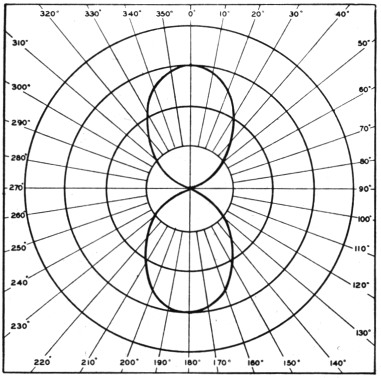
Fig. 2. A plot of A in Table 1 - the horizontal pattern of two vertical radiators spaced one-half wavelength and excited in phase.
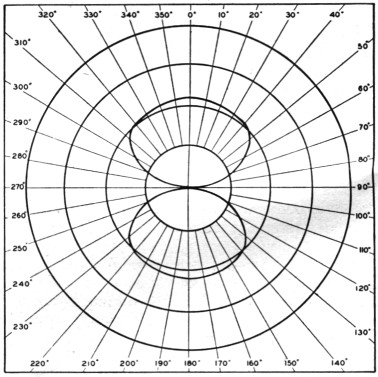
Fig. 3. The horizontal pattern of two vertical radiators spaced one-half wavelength and excited 180° out of phase - B in Table 1.
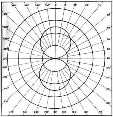
Fig. 4. A plot of C in Table 1 - the horizontal pattern of two close-spaced vertical radiators excited 180° out of phase.
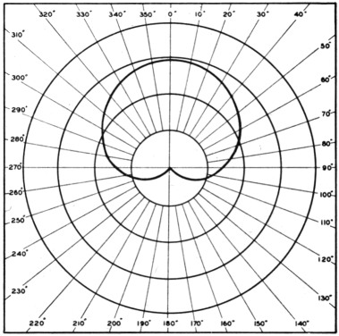
Fig. 5. The horizontal pattern of two vertical radiators spaced one-quarter wavelength and excited 90° out of phase - D in Table 1.
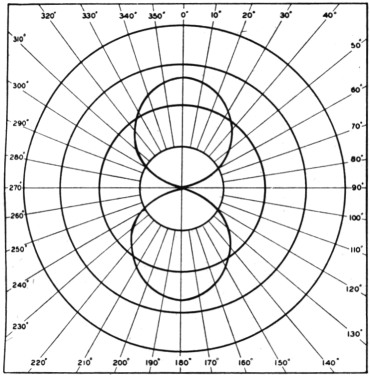
Fig. 6. One of the most fundamental configurations - the horizontal pattern of a horizontal half-wave antenna - E in Table 1.
To find the pattern of two horizontal half-wave elements strung end to end and fed in phase (collinear), the fundamental pattern of the horizontal half-wave element (E) is multiplied in 5° steps by the group pattern of two vertical antennas fed in phase and spaced one-half wavelength (A), as shown by the sample calculations in Table 2. The resultant pattern is shown in Fig. 7. Note that in this and other combinations, it is only necessary to consider the centers of individual elements, their orientation and their spacing in order to use the basic group patterns of A, B, C and D in Table 1.
| Φ | A × | E / 100 = | Pattern of 2 half-wavelength antennas fed in phase and placed end to end | Φ |
|---|---|---|---|---|
| 0 | 150 | 1.345 | 202 | 360 |
| 5 | 148 | 1.34 | 198 | 355 |
| 10 | 145 | 1.31 | 190 | 350 |
| 15 | 140 | 1.28 | 179 | 345 |
| 20 | 129 | 1.22 | 157 | 340 |
| 25 | 120 | 1.17 | 140 | 335 |
| 30 | 108 | 1.11 | 120 | 330 |
| 35 | 92 | 1.035 | 96.2 | 325 |
| 40 | 79 | .945 | 74.7 | 320 |
| 45 | 64.5 | .84 | 54.2 | 315 |
| 50 | 53 | .75 | 39.8 | 310 |
| 55 | 41.5 | .66 | 27.4 | 305 |
| 60 | 33 | .55 | 18.2 | 300 |
| 65 | 24 | .40 | 9.60 | 295 |
| 70 | 15 | .265 | 3.98 | 290 |
| 75 | 7.5 | .185 | 1.39 | 285 |
| 80 | 3.7 | .088 | .326 | 280 |
| 85 | 2.2 | .044 | .0968 | 275 |
| 90 | 0 | 0 | 0 | 270 |
| 95 | 2.2 | .044 | .0968 | 265 |
| 100 | 3.7 | .088 | .326 | 260 |
| 105 | 7.5 | .185 | 1.39 | 255 |
| 110 | 15 | .265 | 3.98 | 250 |
| 115 | 24 | .40 | 9.60 | 245 |
| 120 | 33 | .55 | 18.2 | 240 |
| 125 | 41.5 | .66 | 27.4 | 235 |
| 130 | 53 | .75 | 39.8 | 230 |
| 135 | 64.5 | .84 | 54.2 | 225 |
| 140 | 79 | .945 | 74.7 | 220 |
| 145 | 92 | 1.035 | 96.2 | 215 |
| 150 | 108 | 1.11 | 120 | 210 |
| 155 | 120 | 1.17 | 140 | 205 |
| 160 | 129 | 1.22 | 157 | 200 |
| 165 | 140 | 1.28 | 179 | 195 |
| 170 | 145 | 1.31 | 190 | 190 |
| 175 | 148 | 1.34 | 198 | 185 |
| 180 | 150 | 1.345 | 202 | 180 |
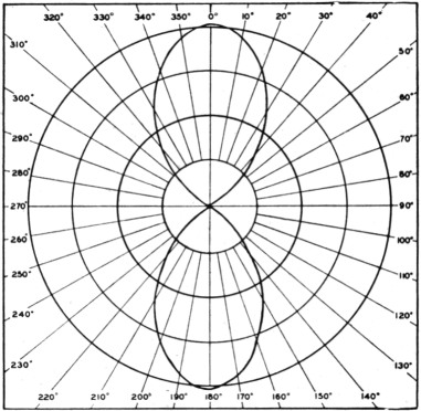
Fig. 7. A plot of the result of Table 2, the horizontal pattern of two collinear horizontal antennas spaced one-half wavelength.
In order to determine more closely in which vertical and horizontal directions the energy is being radiated, it is necessary to multiply in the same manner the horizontal pattern you have just obtained by the ground-reflection factor given in The ARRL Antenna Book (pages 16 through 19) for the particular height at which your array is located. The ground-reflection factor then shows you at what vertical angle the lobe of maximum radiation is directed.
By using combinations of group patterns, particularly the cardioid pattern of Fig. 5 (D in Table 1), many more complicated arrays can be computed. Also binomial arrays - arrays in which lesser currents are fed to the outer elements, for minor-lobe reduction - can be computed. For example, the pattern of a binomial array in which three horizontal elements in line are fed with unit current in the outer elements and twice this current in the center element (all in phase and spaced one-half wavelength) can be obtained by multiplying by itself the pattern of two vertical elements spaced one-half wavelength, fed in phase, and then multiplying the result (approximately a figure 8 squared) by the fundamental pattern of a horizontal half-wave antenna. This is possible because the center element with its twofold current can be considered as two superimposed elements with unit current in each element. This antenna might then be made unidirectional by adding another three half-waves spaced a quarter wavelength from the first set, feeding them in phase with each other but 90° out of phase with the initial set and with unit currents in the outer elements and twice unit current in the center element. This pattern could be computed by multiplying the pattern of the initial three-element section by the pattern for two vertical elements spaced one-quarter wavelength and fed 90° out of phase (D in Table 1).
Other arrangements
The patterns of a good number of arrays can be calculated by the above method, and a little paper work in one's spare time will be found interesting and educational. However, it must be remembered that gain comparisons cannot be readily made with these patterns unless something is known about the impedances of the various elements making up an array, since the only way the patterns can be compared directly to give relative gains is to reduce them to a common basis with equal currents flowing in the elements of the arrays under consideration. If this can be done, by a knowledge of the impedances present, and assuming unit power delivered to each system, a direct graphical comparison can be made. However, some idea of the relative gains can be obtained by visualizing the amplitude of the major lobes if the two antenna patterns under comparison were drawn on such a scale as to have equal total areas.
- And, in greater detail, Grammer, "The all-around radiation characteristics of horizontal antennas," QST, November, 1936, and
Grammer, "More on the directivity of horizontal antennas," QST, March, 1937.
David C. Clecker, W8YBF.