Pi and Pi-L design curves
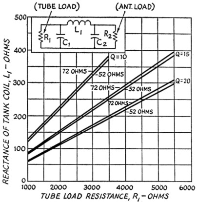
Fig. 1. Reactance of tank coil, L1, as a function of tube load resistance, R1 (for pi networks).
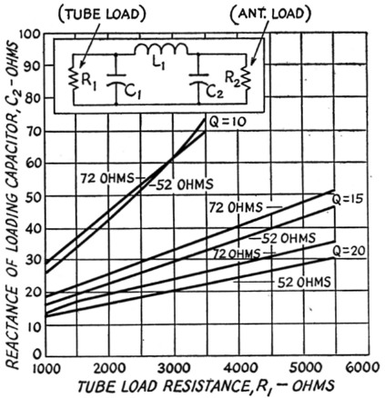
Fig. 2. Reactance of loading capacitor, C2, as a function of tube load resistance, R1 (for pi networks).
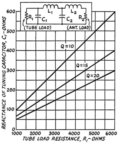
Fig. 3. Reactance of tuning capacitor, C1, as a function of tube load resistance, R1 (for pi and pi-L networks).
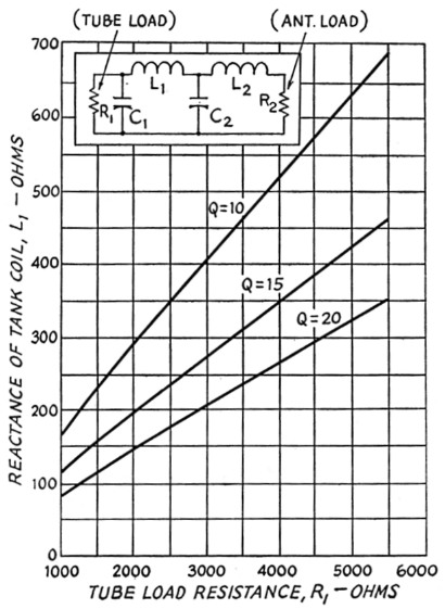
Fig. 4. Reactance of tank coil, L1, as a function of tube load resistance, R1 (for pi-L networks).
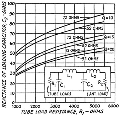
Fig. 5. Reactance of loading capacitor, C2, as a function of tube load resistance, R1 (for pi-L networks).
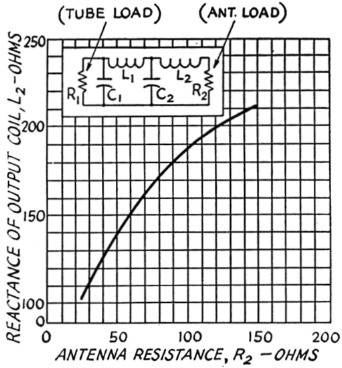
Fig. 6. Reactance of loading coil, L2, as a function of antenna load resistance, R2 (for pi-L networks).
Easy computation of tank-circuit constants.
In a series of charts, this article presents the necessary design data for the popular pi and pi-L tank circuits. Only the simplest arithmetic (and very little of that) is needed for arriving at the proper L and C values.
Since pi and pi-L networks are being used increasingly in transmitter output circuits, the graphs shown here have been prepared in an effort to simplify the design of such tank circuits. The merits of these circuits will not be discussed here since they have been covered in the later references on page 104. Figs. 1, 2 and 3 can be used for determining the values of the components in a pi network while Figs. 3, 4, 5 and 6 can be used for pi-L networks. These curves are drawn for special cases but cover the most generally used operating Qs, tube load resistances and antenna impedances. To use the charts it is only necessary to know the type of tube to be used in the final amplifier, its plate voltage and plate current, the desired operating Q, and the antenna impedance.
Using the pi-network charts
- Choose the power amplifier tube to be used.
- Select the plate voltage and current for normal operation from tube manuals or tables.
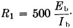
- Determine tube load resistance from R1 = 500 Eby where R1 is the approximate a.c. plate load resistance, Eb is the plate voltage and Ib is the plate current in milliamperes when the amplifier is properly resonated and loaded.
- Determine the operating Q. Operating Q is the Q of the plate circuit when the power amplifier is properly resonated and loaded. Low operating Q means lower harmonic attenuation but better efficiency while high operating Q means better harmonic attenuation but lower efficiency. It is therefore necessary to compromise, and it is considered good practice to use an operating Q between 10 and 20. With the emphasis on reduction of TVI, it might be better to use operating Qs between 15 and 20 and design the tank coils to handle the small additional losses.
- Determine the antenna load resistance. These charts are designed for use with either 52 or 72 ohm loads as these are most generally used and coax cables for these impedances are readily available.
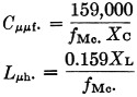
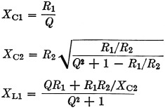
Having made the above decisions, we can find the reactance of the tank coil from fig. 1, the reactance of the loading capacitor from fig. 2 and the reactance of the tuning capacitor from fig. 3. These reactances can be changed to inductances and capacitances at the desired operating frequency by the use of reactance charts or slide rules,(1) or from the following formulas:
| Example: | Power amplifier tubes, two 6146 | |
| Plate voltage | 600 V | |
| Plate current | 200 mA | |
| Operating Q | 15 | |
| Antenna impedance | 52 Ω | |
Then ![]()
Using Fig. 1, we find that the R1 = 1500 ohms line intersects the 52 ohm (Q = 15) line at 112 ohms. Thus the reactance of L1 equals 112 ohms.
Using Fig. 2, we find that the R1 = 1500 ohms line intersects the 52 ohm (Q = 15) line at 19 ohms. Thus the reactance of C2 equals 19 ohms.
Using Fig. 3, we find that the R1 = 1500 ohms line intersects the Q = 15 line at 100 ohms. Thus the reactance of C1 equals 100 ohms.
From the reactance formulas, we find the following at an operating frequency of 3.5 Mc.:
if XL1 = 112 ohms, then L1 = 5 µH;
if XC2 = 19 ohms, then C2 = 2400 pF;
if XC1 = 100 ohms, then C1 = 450 pF
If it is difficult to get 2400 pF for C2, we could let Q = 10 and we would get the following values by using the above process:
XL1 = 170 ohms; L1 = 7.0 µH.
XC2 = 34 ohms; C2 = 1200 pF
XC1 = 150 ohms; C1 = 300 pF
Here is a case where practical considerations in selecting components could dictate the use of lower operating Qs at the lower frequencies.
Using the Pi-L Network Charts
- Choose the power amplifier tube type.
- Select plate voltage and plate current.
- Determine the tube load resistance from
- Choose operating Q.
- Choose antenna load resistance.
Then Fig. 3 gives the reactance of tuning capacitor C1, Fig. 4 gives the reactance of tuning coil L1, Fig. 5 gives the reactance of loading capacitor C2, and Fig. 6 the reactance of loading coil L2.
| Example | Power amplifier tubes, two 4-250As. | |
| Plate voltage | 2500 V | |
| Plate current | 400 mA | |
| Operating Q | 15 | |
| Antenna impedance | 52 Ω | |
Then ![]()
From Fig. 3, XC1 = 210 ohms.
From Fig. 4, XL1 = 285 ohms.
From Fig. 5, XC2 = 53 ohms.
From Fig. 6, XL2 = 144 ohms.
Then at 3.5 Mc. we have the following:
if XC1 = 210 ohms, then Cl = 220 pF;
if XL1 = 285 ohms, then L1 = 13 µH;
if XC2 = 53 ohms, then C2 = 875 pF;
if XL2 = 144 ohms, then L2 = 6.5 µH.
Equations Used for Charts
For pi networks:
For L networks:
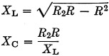
where R is the resistance (higher than R2) to which both the pi and L are matched.
References
- Klippel, "Design considerations for class C power amplifiers," CQ, May, 1950.
- Pappenfus and Klippel, "Pi network tank circuits," CQ, Sept., 1950.
- Pappenfus and Klippel, "Further notes on pi and L networks," CQ, May, 1951.
- Grammer, "Pi-network design curves," QST, April, 1952.
Notes
- Such as the chart in the miscellaneous data chapter in the Handbook, or Figs. 3-83 and 3-84 in the Antenna Book.
R.C. Miedhe, W0RSL.