Designing the VFO
Circuits constants for high stability.
The ever-interesting question of oscillator stability is examined in this article. Although some of the important ingredients of the design formulas are of necessity known only approximately, careful reading will give an insight into oscillator operation that will be of great benefit to the builder who wants to arrive at optimum circuit constants for his VFO with a minimum of cut-and-try.
As a result of continual striving for improved frequency stability, we are confronted today by innumerable VFO types, with spenial virtues being claimed for each. To those contemplating the construction of a VFO this situation can be confusing.
It is not the purpose of this article to compare the various VFO types. The author believes that stable oscillators are more the result of careful design and construction than the use of a particular circuit configuration. The two broad oscillator types which will be discussed are the Colpitts and Hartley circuits. For certain practical reasons the simple Colpitts and Hartley oscillators prove inflexible. The main emphasis will therefore be placed on modifications of these circuits, the Clapp(1) and Lampkin(2) oscillators, respectively.
Feed-back oscillators
The Colpitts and Hartley oscillators belong to the general class of feed-back oscillators. This type of oscillator functions by exciting an amplifier from a portion of its own output. If the amplifier has sufficient gain to overcome the losses in the feed-back loop, oscillation may result.
The usual feed-back oscillator may be represented as shown in Fig. 1A. The amplifier is generally a single vacuum tube. The coupling network feeds back a specified portion of the amplifier output to the input terminals. In general, the coupling network has transmission or phase characteristics such that the circuit is self-exciting at a single frequency. Fig. 1B illustrates how a Colpitts oscillator circuit may be redrawn to conform with Fig. 1A.
Suppose initially that, in Fig. 1A, S1 is opened and that Ein is supplied from an external source not shown. If the coupling network delivers a voltage Efb, identical with Ein, Efb may be substituted for the externally supplied Ein without disturbing the voltages and currents in the circuits. Therefore, if the external source of Ein is removed and S1 closed, the circuit will supply its own excitation and will oscillate continuously.
Two conditions are necessary for sustained oscillations in feed-back oscillators. These are that the amplitude and the phase of the voltage fed back must equal the amplitude and phase of the initially assumed input voltage. Stated in other words, the conditions are a loop gain of unity and a loop phase of zero or 360 degrees.
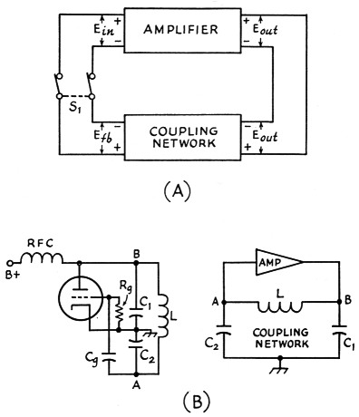
Fig. 1. Feed-back oscillators. A - generalized oscillator; B - Colpitts oscillator circuit (left) and (B) the basic circuit redrawn to show its resemblance to A.
It is unreasonable to suppose that the gain of the amplifier would remain sufficiently constant so that after an initial adjustment the loop gain would forever remain at unity. In practice, feedback oscillators are always designed so that, with the loop opened, the loop gain exceeds unity. When the loop is closed and oscillations begin, some nonlinear circuit element is used to control the loop gain and automatically maintain it at unity.
In the Class C oscillator, the nonlinear properties of the tube stabilize the oscillation amplitude if a grid leak is used to obtain self-bias. When the oscillator is first turned on, the grid bias is zero and the amplifier gain is maximum. In response to any circuit disturbance oscillations will start. The amplitude of these oscillations will grow until the grid bias resulting from the rectifier action between grid and cathode is just sufficient to reduce the loop gain to unity. At this point the amplitude of oscillation will remain constant.
With the relatively high grid bias and a.c. grid voltage peaks in a Class C oscillator the plate current is not a linear function of the grid voltage. It contains, in general, a d.c. component, a component at the fundamental frequency, and many harmonic components. For this reason the coupling network in Class C oscillators usually includes a high-Q resonant circuit. The resonant circuit discriminates against the harmonics and feeds back an essentially sinusoidal voltage, at the fundamental frequency, for grid excitation.
When an oscillator is required to deliver a pure output, free from harmonics, it is usually operated in a Class A condition. In order that the tube may operate as a linear amplifier, it is necessary to use a nonlinear element in the external circuit to control the oscillation amplitude. For instance, it is possible to rectify some of the output of the amplifier and obtain a negative d.c. potential. If this potential is applied to the grid of the amplifier in a suitable manner it will control the amplifier gain in response to oscillation amplitude. The amplifier itself can then operate Class A.(3)
Another example of the Class A oscillator is the Wein Bridge audio oscillator. This circuit uses the nonlinear resistance properties of a lamp filament to control the feed-back in such a way as to maintain the loop gain equal to unity.
The Clapp oscillator
Fig. 2 shows the a.c. conditions in the Clapp oscillator, neglecting for the moment the d.c. connections. C2 is used as the reference capacitor. The capacitances of C1 and C3 are expressed as ratios with C2 by P and K. If P is made zero (corresponding to short-circuiting C1) the Clapp oscillator is reduced to a Colpitts oscillator. Therefore, if design equations are obtained for the Clapp oscillator, it will only be necessary to make P equal to zero in these equations to get the corresponding equations for the Colpitts oscillator.
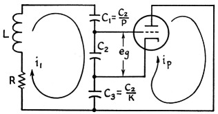
Fig. 2. The a.c. circuit essentials of the Clapp or "series-tuned" Colpitts oscillator.
When the Clapp oscillator is analyzed two equations may be obtained:(4)
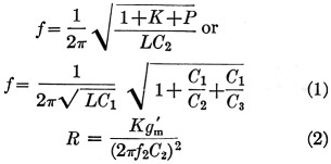
Equation (1) is simply a statement of the resonant frequency of the circuit formed by L, Cl, C2, C3 and R, neglecting any tube effects; the circuit meets the necessary condition of a loop phase of 360 degrees. Equation (2) states the requirements for a loop gain of unity. If the oscillator operates Class A, g'm equals the normal tube transconductance. For other than Class A operation, g'm equals the fundamental component of the plate current divided by the fundamental component of the signal voltage between cathode and grid. It might, therefore, be called the "effective" transconductance. This effective transconductance is always less than the Class A transconductance.
When oscillations exist, Equations (1) and (2) must be satisfied simultaneously. Simultaneous solution yields Equation (3).
Equation (3) is a convenient design equation for the Clapp oscillator. (To obtain the corresponding equations for a Colpitts oscillator we need only make P equal to zero.) It determines C2 in terms of f, Q, g'm, K and P. The choice of values for these constants will be discussed later; for the moment, consider that the values are known. We may then evaluate C2 and therefore C1, C3 and L. The resonant circuit will then be completely determined.
A comparison of the Clapp and Colpitts oscillators
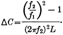
The alternate form of Equation (1) indicates that when the ratios ![]() and
and ![]() are very small the frequency will be primarily determined by L and C3. Since the relatively fickle input and output capacitances of the vacuum tube comprise portions of C2 and C3, respectively, one might feel that the oscillator frequency in the Clapp connection is not as greatly affected by changes in the tube capacitances as would be the case with the Colpitts oscillator. To test this hypothesis it is necessary to determine the rate at which the frequency varies with changes in C2 and C3, for both Clapp and Colpitts circuits. Mathematically, this requires differentiation of Equation (1) with respect to C2 and C3. When this is done we find
are very small the frequency will be primarily determined by L and C3. Since the relatively fickle input and output capacitances of the vacuum tube comprise portions of C2 and C3, respectively, one might feel that the oscillator frequency in the Clapp connection is not as greatly affected by changes in the tube capacitances as would be the case with the Colpitts oscillator. To test this hypothesis it is necessary to determine the rate at which the frequency varies with changes in C2 and C3, for both Clapp and Colpitts circuits. Mathematically, this requires differentiation of Equation (1) with respect to C2 and C3. When this is done we find
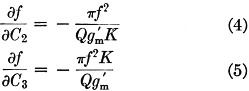
For those not familiar with the calculus, Equation (4) states that, for small changes, the change in frequency is ![]() times the change in C2. For maximum stability, therefore, the factor
times the change in C2. For maximum stability, therefore, the factor ![]() must be made as small as possible.
must be made as small as possible.
This points out the desirability of the highest possible values of Q and gm. Notice that K appears in the denominator of Equation (4) and the numerator of Equation (5). If K is made large to increase the frequency stability with respect to C2 it decreases the stability with respect to C3. This factor will determine our subsequent choice of a value for K.
Since P does not appear in either Equation (4) or (5), these equations apply equally to a Colpitts oscillator. Therefore, if the coil Qs are equal, the stabilities of the Clapp and Colpitts oscillators with respect to tube capacitance changes are identical. Clapp's addition of a third capacitor to the Colpitts oscillator does not improve its frequency stability.5 However, the extra element adds an additional degree of freedom to the oscillator design. We shall use this freedom later in choosing a value for P.
The Lampkin Oscillator
Fig. 3 is a schematic diagram of the Lampkin oscillator. It bears the same relationship to the Hartley oscillator that the Clapp does to the Colpitts. The coil, L, is tapped in the ratio 1, K and P. If it contains N turns, there will be ![]() turns between grid and cathode
turns between grid and cathode ![]() turns between plate and cathode and
turns between plate and cathode and ![]() turns between the grid and the hot end of C.
turns between the grid and the hot end of C.
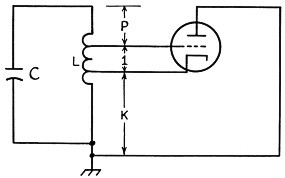
Fig. 3. The Lampkin oscillator circuit.
Using techniques equivalent to those employed in the analysis of the Clapp oscillator the following equations are obtainable for the Lampkin oscillator.
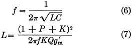
Equation (7) is the design equation corresponding to Equation (3) for the Clapp oscillator. It determines L in terms of the circuit constants. Substitution of the value of L into Equation (6) will yield C and again the resonant circuit design is complete. The analogous equations for the Hartley oscillator are obtained by setting P equal to zero in Equations (6) and (7).
It can also be shown that the stability equations, (4) and (5), apply equally to the Lampkin and Hartley oscillators, where C2 and C3 are now the grid-to-cathode and plate-to-cathode capacitances, respectively.
Electron-Coupled Oscillators
The circuits being discussed are often incorporated into electron-coupled oscillators. E.c.o.s are usually thought of as two-section devices, comprising individually an oscillator and an amplifier with the coupling between them due to the common electron stream. Whether or not this is true depends on the circuit configuration.
Consider the circuit of Fig. 4A. This is a conventional e.c.o. of the Colpitts type with the ground point at the screen grid or "plate" of the oscillator section. The equivalent circuit is shown in Fig. 4B. Notice that the total a.c. tube current flows through the feed-back element C3. This means that the screen and plate currents are both available for feed-back. The plate current predominates because it is larger than the screen current.
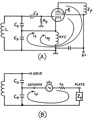
Fig. 4. Grounded plate "electron.coupled" oscillator (A) and (B) its equivalent circuit.
With the average pentode the plate resistance rp is very much larger than the sum of Zp (the plate load impedance) and the impedance seen looking into the resonant circuit across C3. When this is so the plate current is independent of the load impedance, to a first-order approximation. For this reason the frequency of oscillation is relatively independent of variations of the plate load, but it is evident that the e.c.o. of Fig. 4 is not a two-section device. The circuit would therefore be designed in the same manner as any simple oscillator, neglecting Zp. If the ground point in the oscillator is moved to the cathode, as illustrated in Fig. 5, only the screen current flows through the feed-back element. In this case the oscillator section of the e.c.o must be designed using the characteristics of the triode formed by the cathode, grid and screen of the tube.
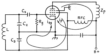
Fig. 5. Grounded-cathode electron-coupled oscillator. The coupling between the oscillator section and output circuit is actually through the electron stream in this circuit, providing there is negligible capacitive coupling between the screen grid and plate. Neutralizing usually is required f'or eliminating such undesired coupling.
Selection of g'm
As indicated earlier, the effective transconductance in Class B or C is smaller than the Class A value. Fig. 6 illustrates the variation of the effective transconductance with grid bias. This graph is the result of a theoretical calculation of gm versus grid bias, assuming that the plate current is a linear function of the grid voltage. While this will never be strictly true, the graph gives a fair engineering approximation. Incidentally, wherever cut-off bias is mentioned in this article it refers to the projected cut-off, and not the actual cut-off bias. This is also illustrated in Fig. 6.
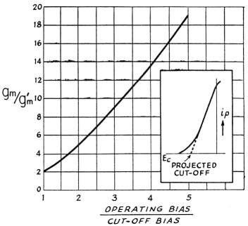
Fig. 6. Approximate relationship between operating bias and effective grid-plate transconductance. The effective transconductance is expressed as a ratio with the normal transconductance of the tube as a Class A amplifier, and the operating bias as a ratio to the projected cut-off bias.
The stability formulas, (4) and (5), show that the frequency stability increases directly with g'm. Therefore, when maximum stability is desired, Class A operation is indicated. As mentioned earlier, Class A oscillators are two-loop devices, and the problems affecting the design of the auxiliary amplitude-controlling loop are a subject in themselves. We shall therefore con eider only oscillators in which the amplitude of oscillation is limited by the nonlinear properties of the vacuum tube.
The desirability of operating with g'm as large as possible suggests that the operating bias should be kept as small as is consistent with the requirement that the gain be effectively controlled. Experience indicates that the operating bias will be the neighborhood of cut-off under these conditions, so that where highest stability is desired g'm can be assumed to be approximately one-half gm. However, in view of manufacturing tolerances in tube constants and the decrease in gm toward the end of the tube's life, as well as other factors, a conservative approach would be to use g'm/3 for initial design purposes.
There are times when an oscillator must be designed to develop a specified output voltage. Because of the essentially peak rectifier action between grid and cathode of the oscillator tube the operating bias is very nearly equal to the peak a.c. voltage between grid and cathode. The peak a.c. voltage between grid and plate will therefore be (1 + K) times the operating bias and the peak a.c. voltage across the entire resonant circuit will be (1 + P + K) times the operating bias. When the desired output voltage is known the required operating bias is readily determined. With a knowledge of the cut-off voltage of the tube and the graph of Fig. 6, the required effective transconductance may be found.
A choice of g'm in Class C operation could also be made on an efficiency basis. Terman shows that the optimum length of the plate current pulse, in electrical degrees, is between 120 degrees and 150 degrees for operation at the fundamental frequency. In electron-coupled oscillators, where the plate circuit may be tuned to a harmonic of the oscillator frequency, the optimum angle of plate current flow depends upon the desired harmonic. Terman indicates that the optimum angle is 90 degrees to 120 degrees for the second harmonic, 80 degrees to 120 degrees for the third, and 70 degrees to 90 degrees for the fourth. The corresponding value of g'm may be obtained from the graph of Fig. 6 by first finding the ratio of the operating bias to the cut-off bias from Equation (8):
![]()
As an example, if the desired angle of flow is 90 degrees, cos 1/2 Φp = 0.707. The ratio of operating bias to cut-off bias is therefore 3.42. From the graph we find the effective transconductance is 1/11 the normal transconductance at this point.
Another factor involved in the discussion of g'm is the choice of a vacuum tube type. When stability is important it would appear that the best tube would be that with the highest gm. This is not categorically true. We could always double gm by using two tubes in parallel. Would this increase the stability? The answer is no. While the gm is doubled, so are the tube capacitances and their resultant instabilities; therefore we just break even.
In the writer's view, the best choice is a tube with a high figure of merit, where figure of merit is defined as the gm divided by the sum of the input and output capacitances of the tube. The pentodes used in television r.f. and i.f. circuits are usually tubes with high figures of merit.
Choosing K
The factor that adjust the feed-back ratio is K. In so doing, it also sets the ratio of impedances presented by the resonant circuit between grid and cathode and plate and cathode. The choice of a suitable value for K therefore depends upon the relative stabilities of the input and output impedances of the tube.
If the input and output capacitances of the tube were subject to equal random deviations, a comparison of the stability equations, (4) and (5), indicates that the optimum choice of K would be 1. In typical pentodes, however, the grid capacitance is about ten times less stable than the plate capacitance. Therefore, the normal random deviations in these capacitances will produce the least frequency deviation if K = √10 or about 3.
Selection of P
Earlier, in discussing the stability equations, the value of P was found not to affect the frequency stability of the oscillator. If it does not affect frequency stability we are free to choose any convenient value for P. A convenient value may be determined by considering the resonant circuit design in a VFO from a practical viewpoint.
The object of the resonant circuit design in the average VFO is to produce an oscillator that will tune between two frequencies, f1 and f2, using the maximum rotation of the variable air condenser. That is, maximum bandspread is desired.
The initial conditions imposed on the resonant circuit are two: the tuning range, f1 to f2, and the value of variable capacitance ΔC. When a given frequency range must be covered by a specific variable capacitor, the values of L and C are predetermined.
In the Colpitts and Hartley oscillators the resonant circuit yielding maximum stability is determin 'd by the circuit constants Q, g'm, and K. It is therefore only a fortunate accident when a commercially obtainable variable air condenser is found which, without modification, will simultaneously satisfy the requirements for band-spread and maximum stability.
In the Clapp and Lampkin oscillators the resonant circuit is controlled by Q, g'm, K and P. Since the frequency stability is unaffected by the value of P we can choose values of Q, g'm, and K yielding maximum stability and then choose P so that the oscillator will cover the desired frequency range with whatever variable capacitor is available. The advantage of the Clapp and Lampkin oscillators resides in this ability to match a particular resonant circuit to a specific tube in a manner resulting in maximum frequency stability.
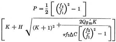
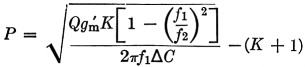
When the frequencies between which the oscillator is to tune and the size of variable capacitor are known, it is merely a mathematical exercise to arrive at the proper value for P.(6) For a Clapp oscillator having a frequency ratio of 1.14 to 1 (the ratio covered by the 3.5-4 Mc. band), P may be found from the following simplified equation, in which K is selected to have the value 3:
![]()
In this equation f2 is the highest frequency to which the oscillator is to tune, and ΔC is the change in tuning capacitance between the maximum and minimum settings.
The value of P may be found in other ways. In the Clapp oscillator, if C2 is arbitrarily selected P may be found from Equation (3). If L is arbitrarily chosen P may be found from Equation (7). Lastly, P itself may be arbitrarily selected. In any of these cases it is of interest to find the value of variable capacitance required to tune between f1 and f2.
In the Clapp oscillator we design around the upper frequency f2. At the lower frequency, f1, P will have a new value P1
![]()
and
![]()
This value of variable capacitance probably will not be commercially available and ΔC must then he tailored to fit, by appropriately modifying a standard variable capacitor - usually by removing plates from one initially too large.
In the Lampkin circuit P may also be selected arbitrarily or found by Equation (7) if L is initially chosen. The required value of variable capacitance is then
Estimating Q
The factor whose value remains to be estimated is Q. An average oscillator coil of good construction will have a Q somewhere between 100 and 300. The Q in the formula is actually the oscillator circuit Q, including all loading effects. In a well-designed circuit which is not required to deliver power (except that consumed by the grid) the circuit Q will very nearly equal the coil Q.
If the Q of a coil using the proposed construction cannot be estimated closely from prior knowledge, a trial value of Q can be assumed and used in finding L. The coil may then be wound and its Q measured. If the measured Q differs from the assumed Q, a new calculation for L can be made using the measured value of Q. With similar construction the Q of the second coil will be very close to the measured Q of the first.
In case facilities for measuring Q are not available, its value should be estimated on the conservative side. This will ensure oscillation, and after the oscillator is constructed the capacitances of C2 and C3 may be increased to the point where the largest usable value of P is reached, if desired.
Grid capacitor and resistor
In the actual construction of the oscillator an RC grid-leak combination must be selected. The value of the grid capacitor should be made much larger than the input capacitance of the tube so that the voltage across C2 will actually appear between grid and cathode of the tube. Rg should be made as large as possible to minimize the effective grid loading on the resonant circuit. However, if the time constant of the RC combination becomes too large, intermittent oscillations will result. As an initial compromise, Cg is usually made about 10 times the input capacitance of the tube. Rg is then selected so that the time constant of RgCg is 10 times the period of the highest operating frequency. That is:
![]()
After the oscillator is working properly the resistance Rg is raised to as high a value as is possible without causing intermittent oscillation.
Concluding Remarks
The design procedure for VFOs outlined in this article is one which minimizes the effects of vacuum tube instabilities on the oscillator frequency. While the short-term stability of an oscillator depends to a great extent on vacuum-tube fluctuations, long-term stability is a function of several other factors. Among them are attention to mechanical detail and the effects of temperature on the oscillating circuit constants.
It is not difficult to achieve short-term stabilities of a part in 105, or better, with the vacuum tubes currently available. In contrast with this we find that the average VFO has a mechanical resetability of about one part in 103. Normal temperature variations cause frequency drifts of about one part in 104 even in "temperature compensated" VFOs. In a well-balanced design the ratio between the long-and short-term stabilities should not exceed ten. With the present state of the art this balance can be achieved only by paying meticulous attention to mechanical design and construction, and to temperature compensation. Ponder awhile on this fact before you begin the design of a VFO to obsolete all other VFOs.
Appendix
From impedance considerations in the oscillator loop it can be shown that when a Clapp oscillator is designed for some specific frequency f1 and C1 is varied, the loop gain increases as the frequency of oscillation decreases. In the Lampkin oscillator the reverse is true. Therefore, to insure that oscillations will exist over the entire frequency range, the Clapp oscillator should be designed around the upper frequency f2, and the Lampkin around the lower frequency f1. When this is done the value for P in the Clapp oscillator is given by
For the Lampkin oscillator, P is given by
The latter equation shows that there is a possibility of obtaining a negative value for P in the Lampkin oscillator. This possibility occurs when the impedance of the resonant circuit dictated by ΔC, f1 and f2 becomes too low to support oscillation. If this occurs the value of ΔC should he reduced until P becomes positive.
Notes
- Clapp, "An inductance-capacity oscillator of unusual frequency stability," Proc. I.R.E., 36, 356-358 (1948).
- Lampkin, "An improvement in constant frequency oscillators," Proc. I.R.E., 27, 199-201 (1939).
- Bernstein, "Amplitude limiting for the VFO," QST, Feb., 1954.
- Proofs of these and subsequent equations accompanied the manuscript, but are not included here since they have been given (in slightly different form) in other papers; e.g.,
Gouriet, "High-stability oscillator," Wireless Engineer, April, 1950. - Ed; - In practice it would be difficult, although perhaps not impossible, to construct a low-inductance coil for the "high-C" Colpitts or Hartley having as good Q as a coil of the larger inductance typical of the series-tuned Colpitts, within the same physical dimensions. Also, impractical values of variable capacitance are required in the Colpitte and Hartley circuits at the lower frequencies.
- See Appendix for complete design equations.
Louis Howson, W2YKY.