Optimum stacking spacings in antenna arrays

Home - Techniek - Electronica - Radiotechniek - Radio amateur bladen - QST - Optimum stacking spacings in antenna arrays

Effect of source beam width on stacking.

When the "elements" of an antenna array are in themselves beam antennas, as in multiple-Yagi antennas, the question of the optimum stacking spacing becomes of very great interest. Available data covers principally stacked dipoles. This article outlines the principles and presents essential design information in two graphs.

During antenna discussions one often hears the remark that stacking two antennas results in a 3 dB gain improvement. Actually, a more accurate statement is that stacking two antennas can result in a 3 dB gain improvement if the proper spacing is chosen. The latter part - i.e., the proper or optimum spacing idea - has been grasped at by many amateurs. For instance, W2PAU(1) and W2NLY(2) have found that a spacing greater than ½ wave length is needed in order to achieve maximum gain from multiple-element arrays.

The Handbook and other literature point out that maximum gain for two collinear dipoles occurs at approximately ¾ wave length spacing. Mention is also made of the fact that large spacings are needed with high-gain Yagis in order to obtain an appreciable increas in gain. The usual explanation for this increase in gain is that the "capture area" has been increased.

Before going on, two important points need clarification. The first of these is the 3 dB gain improvement associated with stacking two elements of an array. This result is the misuse of the often quoted formula for power gain:

where A is the area and λ is the wave length. Hence, if we double the area the power gain is doubled. The relative increase in dB is then given by

This formula was derived for a uniformly-illuminated aperture. In practice, this condition is approached in certain types of antennas. However, it should be evident that the term "area" implies physical area. An array of a large number of dipoles presents a physical area and a corresponding gain. Doubling the physical size of the array does double the power gain. In contrast, a single dipole has very little physical area, and if any geniuses think that doubling the wire diameter will double the area and the power gain - well, they might as well go back to their stringless yo-yo's. This brings up our second point, which is "capture area."

Directivity and gain

The concept that "area breeds gain" leads one to ask how a dipole, which has an insignificant amount of physical area, obtains its gain. Here we must revert to even more-fundamental concepts. The first is that of directivity, D, defined(3) as the ratio of the maximum radiation intensity from a given source to the radiation intensity from an isotropic source radiating the same total power. (An isotropic source is one that radiates energy uniformly in all directions.) Directivity can also be expressed as

where the beam area B is the solid angle through which all the power radiated would stream if the power per unit solid angle equaled the maximum value over the beam area. For pencil-beam antennas

where θ1 and φ1 are the half-power beam widths, in radians, in each plane. This results in the often-used "gain" equation,

where θ1 and φi are now in degrees.(4) Power gain is defined as

where k is an efficiency factor and is equal to 1 for a lossless antenna. The concept of directivity is universal in that it is strictly a function of the antenna pattern and is independent of losses.

By comparing(5) the maximum radiation intensity of a dipole with the radiation intensity of an isotropic source radiating the same total power, and assuming a lossless antenna, we arrive at the magic figure of 2.14 dB, which is the gain of a dipole over an isotropic source.

Effective aperture

So far we have shown why a dipole has gain, but the question of area remains. This requires another concept similar to that of "capture area." Kraus calls it "effective aperture," and defines it as the ratio of the power in the terminating impedance to the power density of the incident wave. If the terminating impedance is adjusted to produce maximum power transfer (the reactances of the load and antenna cancel, and the resistances are equal), and the antenna is lossless, this ratio is called the "maximum effective aperture" (A_em). By more skillful mathematical manipulation we obtain, for a dipole,

Hence, the maximum effective aperture of the dipole is approximately the same as an area ½ by ¼ wave length on a side. The physical significance of this aperture is that power from the incident plane wave is absorbed over an area of this size by the dipole and is delivered to its terminating resistance. The directivity of any antenna is related to its maximum effective aperture by the formula

Now that we have attached a fictitious physical area to any physically small antenna another question arises (problems, always problems!). Since the effective area represents a so-called power-gathering area, how should dipoles or Yagis be spaced for maximum utilization of their respective A_em's? Unfortunately, while the formulas above point the way, they do not give the answer. Although formula (7) shows the item of a dipole to be approximately equal to an area ½ × ¼ wave length, other geometric figures (ellipse, circle, etc.) could just as well be used, so long as the area is equal to 0.13 λ². Likewise, formula (8) shows that as the directivity of an antenna increases (as it does when more directors are added to a Yagi) its maximum effective area increases correspondingly. This suggests that the stacking spacing should also keep increasing.

Pattern multiplication

To show that this is so, and also to determine the optimum spacing for maximum gain, the author employed the principle of pattern multiplication.° It states that the field pattern of an array of nonisotropic but similar point sources (i.e., an array of dipoles, or Yagis, or horns, etc.) is equal to the field (voltage) pattern of the individual source multiplied by the field pattern of an array of isotropic point sources having the same locations, relative amplitudes, and phases as the nonisotropic sources. It should be pointed out that to be called "similar," the patterns of the individual sources must not only be of the same shape, but must be oriented in the same direction. Although these sources may be of finite size (like Yagis) each can be considered to be a point source situated at the point in the antenna to which phase is referred. Fig. 1 illustrates a simple case of four collinear dipoles.

Fig 1
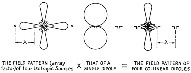
Fig. 1. Illustrating the principle of pattern multiplication.

The field pattern of the isotropic sources at various spacings and phases is called the "array factor." Hence, by taking the field pattern of one element of an array (consider two stacked elements, i.e., n = 2, where one element has a 30° half-power beam width in the stacking plane) and multiplying by the various array factors corresponding to the spacings chosen, a series of patterns results as shown in Fig. 2. These patterns are the same far-field patterns you would get by stacking two 30° Yagis at the spacings shown (assuming your feeders don't radiate!).

Fig 2
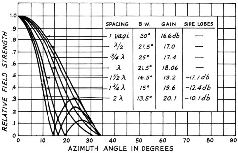
Fig. 2. Theoretical field patterns and gain vs. spacing for two Yogi sources having ha If-power beam widths of 30 degrees, fed in phase.

Gain vs. stacking spacing

We now have a series of patterns plotted to the same relative scale, and we want to determine which pattern results in maximum gain. Previously we saw that for a 100 per cent efficient antenna the directivity is equal to the power gain, and that the directivity is simply a measure of the antenna's beam width. By measuring the beam widths from the patterns and using the proper beam width in the opposite plane, we can calculate D and, finally, db. gain.(7)

These gain figures are valid, but only to a certain point. By looking closely at the trend of the patterns for two collinear dipoles shown in Fig. 3, we see that as the stacking spacing is increased a point is reached where the side lobes approach equality in magnitude with the main lobe. But even before this happens we are "wasting" power and gain (actually redistributing the power in multiple lobes), and eventually a point is reached where diminishing beam width not only is no longer synonymous with increasing gain, but the gain actually decreases. The author has taken a -10 db. side-lobe level as the change-over point. In some applications side-lobe level is an important, if not the dominant, factor in array design.(8) However, in our case we are simply dealing with sources that are fed in phase and with equal amounts of power.

Fig 5
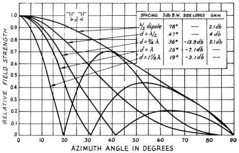
Fig. 3. Field pattern of two-element collinear dipole array.

By drawing the resultant patterns of an array for various element beam widths, and by varying the stacking spacings, the author arrived at Fig. 4. The curves hold for two stacked elements (sources) such as two Yagis.(9)

Fig 3
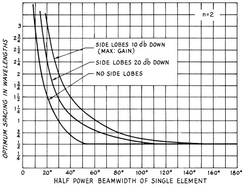
Fig. 4. Optimum stacking spacing for two sources (n = 2). The spacing for no side lobes, especially for small beam widths, may result in almost no gain improvement with stacking.

When the number of elements stacked in an array is increased (individual-element beam width kept constant), the array factor changes. To see what effect this has on the curves given in Fig. 3, the same procedure was used for four elements and the result is shown in Fig. 5. As the number of elements is increased, the array factor pattern becomes replete with minor lobes, and the process of drawing the resultant patterns is no longer a simple task. Because of this, curves were drawn only for n = 2 and n = 4. Optimum spacings for other values of n can be "guesstimated" from Figs. 3 and 4.

Fig 4
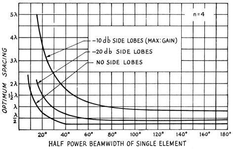
Fig. 5. Optimum stacking spacing for four sources (n = 4). Note: Spacings less than % wave length are physically possible only for shortened dipoles in the case of collinear elements.

Conclusions

A number of interesting conclusions can be drawn from the curves and figures:

For narrow-beam Yagis (approximately 40° and less) the "E" and "H" plane beam widths are approximately equal 1° and the optimum stacking spacings are the same in either plane.
For a given beam width, increasing the number of elements (sources) increases the optimum stacking spacing. Smaller beam widths require a relatively larger increase.
For a collinear array of four elements, it is impossible to obtain a pattern without side lobes until the beam width of the individual end-fire elements comprising the array is less than about 28°. For higher values of n, the zero side-lobe condition occurs only for smaller beam widths.
Appreciable gain is sacrificed by designing for a -20 dB (or lower) side-lobe level, especially when the individual elements have small beam widths.
As deduced from the maximum effective aperture concept, high-gain elements require larger spacings in order to achieve any appreciable increase in gain.
It's a tough job no matter how you look at it.

It is always nice to be able to back a theoretical discussion with experimental evidence. Delving back into the September, 1956, issue of QST,(11) we find patterns and gain figures for a two-element array. The "individual sources" are three-element Yagis stacked in the "H" plane (vertically). Referring to Part 1 of the article,(10) the H-plane beam width of a three-element Yagi is approximately 75°. Looking at our Fig. 3, maximum gain should occur when the two Yagis are spaced a little over ¾ wave length apart. That this is indeed the case is pointed out in the Yagi article.

The generality of Figs. 3 and 4 should not be overlooked. These curves are useful for a dipole or Yagi array or for any type of antenna element, providing the elements are similar. They provide a quick and simple method of optimizing array design.

In practice, slight deviations from the theoretical are quite common. In our analysis, these deviations can be attributed to the assumptions that the elements have no side lobes, are lossless, and the effect on gain of mutual impedance is small. The assumption that the radiation pattern of an individual source does not change in the presence of others leads to errors in pattern shape at low levels of radiation (below -20 db.).

Notes

Brown, "The Wide Spread Twin Five," CQ, March, 1950.
Kmosko, "More Gain with 30 Elements," CQ, November, 1950.
The subject of gain is well covered in Antennas by J. D. Kraus, published by McGraw-Hill, New York City.
Example (from Kraus, op. cit.): for 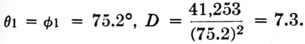For this example the error is about 10 per cent. The error decreases with decreasing beam width.
This comparison is done mathematically by integration.
Kraus, op. cit., p. 67.
D as given by equation (5) is for pencil-beam patterns. For the special case of doughnut type patterns a much better approximation is given by 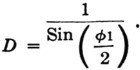The gain (2) figures given should not be taken as absolute values. Of more importance is their relative value for various spacings.
In such cases other schemes are used to reduce the side-lobe level, the most common being the tapered-illumination method, i.e., the magnitudes of the element currents are set in a prescribed fashion. The DolphTchebycheff distribution is the most popular, since for a given side-lobe level, it gives the smallest possible beam width.
The individual source patterns used had no side lobes. The results hold very well even with -10 db. side lobes since the multiplication process tends to reduce them.
Greenblum, "Notes on the development of yagi arrays - Part 1," QST, August, 1956, Figs. 3 and 4. The "E" plane is the one containing the individual radiators comprising the source or element and the "H" plane is at right angles to the axes of the radiators.
Greenblum, "Notes on the development of yagi arrays - Part 2," QST, September, 1956.

H. W. Kasper, K2GAL.