New thresholds in V.H.F. and U.H.F. reception; The world below KTB
Most amateurs are aware that spectacular advances are being made in r.f. amplifier design that promise markedly improved reception throughout the v.h.f. and u.h.f. portions of the spectrum. Here two well-known v.h.f. men who have been active in the development of the reactance amplifier show why the lower noise figures now being achieved are of such importance. A future article will deal with the practical aspects of the new amplifier techniques.
Ever since the first ham twiddled with the first coherer, we have been trying to improve our receivers. Now, with the coming of the maser and reactance amplifier, there appears to be a possibility of an improvement, and in an area where it will do the most good: the frequencies above 100 Mc. In a later article, we will discuss the details of these devices, but now let us back up a bit and consider just what limitations exist in the detection of weak signals and what these devices will buy us. Some of the factors involved are not readily apparent.
Most of us are familiar with the idea of noise figure, as simply a measure of how much worse our receiver is than the ideal receiver. The ideal receiver, in turn, is a device which adds no noise to that fed into it by the antenna.
Noise figure as measured on a noise generator has usually been a criterion of receiving performance, so let's start with it. Such a measurement has just been made and found to be quite good. We are now ready to go on the air so the receiver is connected to the antenna. If everything is matched, there is no reason to believe that the receiver noise figure is now any different, and it isn't. Now assume that the antenna is putting out vast amounts of noise which add to the receiver noise. Obviously, our ability to receive weak signals has suffered, but the noise figure remains the same. What, then, is the paradox? There is none. Noise figure, as considered above, is a measure of the receiver alone.
Apparently, then, noise figure as normally measured does not tell the whole story. To know where we stand, include the effects of the antenna and think in terms of an over-all or effective noise figure. Taking the liberty of one little equation, the relation of a new over-all noise figure, Fo, to the easily measured receiver noise figure, FR, is readily seen:
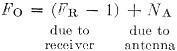
Note that the contribution from the receiver now appears as receiver noise figure minus 1. This unit of 1 was subtracted because it is not part of the actual receiver contribution, but simply the standard of comparison by which the receiver was gauged. It happens to be the thermal noise of the terminating resistor in the noise generator. The equation may be developed by starting with the receiver connected to the noise generator and measuring FR. With the noise generator termination, the effective noise figure, Fo, is simply FR. Now switch the receiver from the generator to the antenna, losing the one unit of noise caused by the termination and adding in its place antenna noise, NA. Hence, Fo is now equal to (FR - 1) + NA. Note that in the above equation if the antenna noise is equal to one, we are back where we started and the over-all noise figure is equal to receiver noise figure.
However, in the more likely event that NA is different than one, the over-all noise figure can be either greater than or less than the receiver noise figure. In fact, the over-all noise figure can even be less than one (negative db.'s), something not possible for receiver noise figure, which by definition includes one rather arbitrary unit of room temperature thermal noise. Thus, if antenna noise is much larger than the receiver noise, obviously we are stuck with it and little over-all improvement can be had by improving the receiver noise figure. For example, with a decent antenna, at 3.5 Mc, it doesn't matter much if the receiver has a 3-db. noise figure or a 6 dB noise figure. Atmospheric noise is so great that doubling the noise generated in the receiver is like adding two watts of additional power to a 500-watt transmitter instead of adding one watt. Your DX contact will never know the difference.
On the other hand, as will be seen, if antenna noise is much less than receiver noise, we really have something to gain by improvements in the front end. A 3 dB improvement in front-end noise figure can result in more than a 3 dB overall improvement. Suppose that you have a receiver with a noise figure, FR, of 2.5 (4 dB), and that antenna noise, NA, is equal to 0.25. The over-all or effective noise figure is 2.5 - 1 + 0.25 = 1.75 (2.4 dB). If the receiver noise figure is now reduced by 3 dB to -1.25 (1 dB), the effective noise figure becomes 0.5 (-3 dB), a net improvement of 5.4 dB. This all seems to prove that sometimes a db. is not a db.
Since antenna noise is a vital factor in the problem, it is worthwhile to take a look at what causes it and what control, if any, we have over it. Antenna noise may be visualized to be thermal noise in a resistance, the radiation resistance of the antenna in question. Its magnitude is :dependent not on the temperature of the physical structure of the antenna, but rather on the effective temperature of whatever the antenna is looking at. (Effective temperature is the product of the actual temperature and a radiation coupling factor.) Thus, the antenna may be considered to be nothing more than a thermometer whose output (noise) is proportional to its "temperature." When such an antenna looks at the open sky above 20 Mc.; we find that it registers an output corresponding to considerable temperature, depending on the direction and frequency in use. This is known as cosmic noise 1 and is the basis of radio astronomy. Fairly complete maps, plotted as power or temperature, have been made of this radiation from the sky, and it is of interest to note that they bear little relation to what we see in the sky visibly.
How intense is this radiation, and how does it vary with frequency? Fig. 1 shows a plot against frequency of the average cosmic noise level (average of all directions) and it can be seen that it is quite high in the h.f. region, has dropped to be equal to room temperature thermal (KTB) at about 175 Mc, and drops to quite low values at u.h.f. For convenience, figures are given in decibels, while the equation was in terms of power ratios.
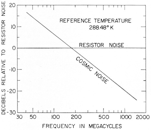
Fig. 1. Average cosmic noise variations with frequency.
It is of interest also to see how this noise varies across different portions of the sky at a given frequency. Fig. 2 shows a plot of the received noise that would be obtained at 144 Mc. with an antenna of 18° beamwidth scanning across the sky at a declination of -30°. (Declination is simply celestial latitude.) This particular sector gives a higher average than the entire sky, but was chosen to show that large variations in level are possible. It would not be necessary to rotate the antenna to obtain this curve, but rather the antenna could be fixed and readings taken over 24 hours while the earth rotates. This curve points up the importance of pointing toward the cold portions of the sky on frequencies where cosmic noise is the limitation, or of waiting until a cold portion is in the direction we wish to work.
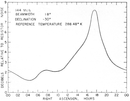
Fig. 2. Example of cosmic noise variation across the southern sky.
We have now seen that overall sensitivity is strongly affected by antenna noise. We have also seen how this antenna noise varies with frequency and antenna direction. Now let us plug in some numbers and see what it all adds up to.
Fig. 3 is a plot of over-all effective noise figure (Fo) versus frequency and includes the effect of both the receiver noise figure (FR) and the cosmic noise level (antenna noise), NA. Three curves are shown, the top one assuming the best available tube noise figures below 500 Mc (416B), and best crystal noise figures above 500 Mc. The middle curve indicates what may be expected with a 1 dB noise figure across the frequency range, and the lower curve gives the result for a perfect receiver or 0 dB noise figure. Note how a small reduction in noise figure is increasingly important at the higher frequencies.
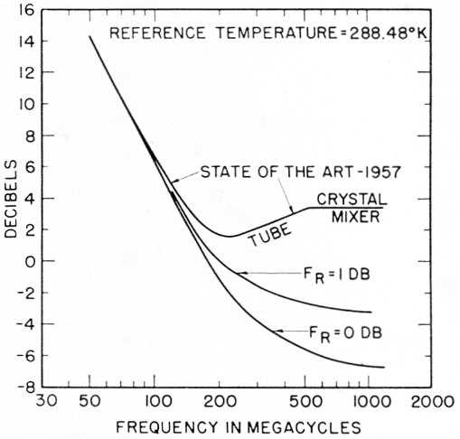
Fig. 3. Over-all effective noise figure for an antenna pointing at the horizon and average cosmic noise.
Fig. 3, it should be pointed out, is based on average cosmic noise (Fig. 1), and therefore does not represent the best conditions. Also, there are certain other limiting effects that must be considered in a practical case and which cause the two lower curves of Fig. 3 to level off rather than to continue downward as does the cosmic noise curve.
First is line loss; you simply can't afford to have very much. Anything that dissipates power also contributes thermal noise. This leads us to consider the use of pole-top front ends or, at u.h.f., waveguides. Also, we must take into account the effects of atmospheric absorption - its attenuation contributes some thermal noise. For the conditions assumed in Fig. 3, it becomes severe only above about 1000 Mc. Solar noise can be overwhelming when we are dealing with low levels and we must avoid the sun with our antenna beam. Hotspots of cosmic noise (radio stars) should also be avoided. Ohmic losses in the antenna must also be minimized due to their resistive noise.
Perhaps the most serious of all is the effect of the ground in front of the antenna. If it is a perfect reflector, there is no problem as it can contribute no noise. However, there is always some loss from ground reflection. This loss looks like a room temperature attenuator and contributes noise. (It is of interest to note that horizontal polarization gives considerably less ground noise contribution than vertical.) The best way to beat it would be to simply have a perfect ground, such as a copper sheet two miles across! If this is not feasible, the next best thing is to tilt the beam up away from the earth; fine for lunar and high-angle meteor work. However, for tropospheric scatter, you will take a beating in doing this because of the increased scatter angle. Even with the antenna tilted up so as to avoid the ground in the main lobe, we still expect some additional noise from side and back lobes which illuminate the "noisy" earth.
Fig. 3 was computed on the basis of representative values of these factors that might be experienced in a typical case.
It is also of interest to consider the best possible situation. This corresponds to viewing the coldest portion of the sky and operating with the antenna tilted up from the ground to eliminate the main-lobe ground contribution and the majority of the atmospheric loss. The over-all effective noise figure under these conditions is shown in Fig. 4 for a zero db. noise figure receiver. It can be seen to represent improvement over present equipment of 3 db. at 144 Mc., 6 db. at 220 Mc., 12 db. at 430 Mc., and 15 db. at 1300 Mc. At 144 Mc., this improvement may be just enough to put us in business with regular moon-bounce contacts. It also corresponds to doubling the burst rate observed in meteoric work.
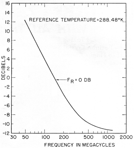
Fig. 4. Over-all effective noise figure for an antenna pointing at a "cold" region well above the horizon.
At the higher bands, the improvement is considerable. The table below takes this improvement and translates it into what may be expected on tropospheric scatter, meteor rate, and lunar echoes, for the power and antennas indicated. It is assumed that c.w. is used with narrow-band receiving techniques.
| 220 Mc | 432 Mc | 1300 Mc | |
|---|---|---|---|
| Antenna Power | 150 W | 150 W(2) | 150 W |
| Antenna Gain over Dipole | 24 dB (24' dish) | 23 dB (17' dish) | 27.5 dB (9½' dish) |
| Tropospheric(3) Scatter Range | 425 mi. | 440 mi. | 365 mi. |
| Meteor Rate | 1.8/min | 0.9/min | 0.13/min |
| Moon Echo, add. system improvement required | 7 dB | 1.5 dB | 0 dB |
For power outputs of 150 watt and modest size antennas, we find that consistent tropo-scatter ranges of nearly 400 mile are to be expected on all three bands. Meteor rates, although dropping rapidly, still indicate about one burst every 7-8 minutes at 1300 Mc. Moon echo work may just be feasible at 1300 Mc as the calculations indicate it is on the ragged edge. Increases in power and antenna size beyond the values indicated should make these higher frequency bands even more attractive. It is evident that with the very low noise figures which are now within reach in amateur practice, performance may be expected on the higher bands that equals or exceeds that on 2 meters.
Notes
- Below about 20 Mc, antenna noise does not consist exclusively of cosmic noise, but is largely caused by such unexotic sources as atmospherics, neon signs, electrical appliances, etc.
- Of academic interest only due to the present 50 watt limitation.
- For tropo we are forced to beam toward the horizon and hence accept some degradation dice to ground noise in the main-lobe and atmospheric loss. This is significant only on 1300 Mc, however.
Ross Bateman, W4AO
Walter F. Bain, W4LTU