"A do-it-yourself" guide to design and construction of log periodic antennas
A new look in antenna structures results from the application of the log periodic concept in antenna design.
This new family of antennas exhibits pattern and impedance characteristics which are essentially frequency independent over extremely wide bandwidths. Ten-to-one bandwidths are readily attained in practice. Various configurations can provide vertical or horizontal linear polarization as well as circular polarization. Radiation patterns can be made uni-, bi-, or omnidirectional with relative ease. This paper shows how to design practical antennas for amateur use at low cost and includes several practical sets of working construction dimensions.
On reading over several articles by R. H. DuHamel(1) disclosing a completely new concept in wide-frequency-range antennas, designing and building one appeared to be a fine project for the "do-it-yourselfer."
The performance of this new antenna structure has now been well established, and sufficient design information has been published to permit one to design a structure for amateur use. The non-frequency-sensitive aspect - the antenna can operate over more than a 10-to-1 frequency range - is the most valuable feature to us amateurs. It is possible, for example, that one antenna could be designed and built to operate over the entire frequency range from 3.5 through 30 Mc using only one feed line, with uniform gain and beam pattern for any frequency within these limits. The v.s.w.r. would average about 1.5:1, with a maximum of 2:1. The available gain will, of course, vary with the beam pattern desired but will run from 5 to more than 10 dB over a dipole. For instance, if a vertical coverage of 90 degrees and azimuth coverage of about 65 degrees is acceptable, a gain of about 6 dB can be attained (cutoff points are assumed to be at half-power levels). The impedance will be within the range 50 to 200 ohm.
All is not gold that glitters, however, and a word of caution must be given that it is essential that a harmonic-rejecting coupler be used between the transmitter and this antenna. The antenna is ready and willing to accept harmonics and other spurious emissions and to radiate them with the same 6 dB gain as the fundamental: Lids, beware! You should use a coupler with any antenna in any case.
A view of a scale model log periodic antenna is shown in Fig. 1, and the dimensions entering into the design are shown in Fig. 2.
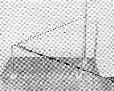
Fig. 1. A u.h.f. model of the log periodic antenna built for pattern measurements. This shows the element configuration that is characteristic of all antennas of this type. This model covers the frequency range from 450 to 5000 Mc.
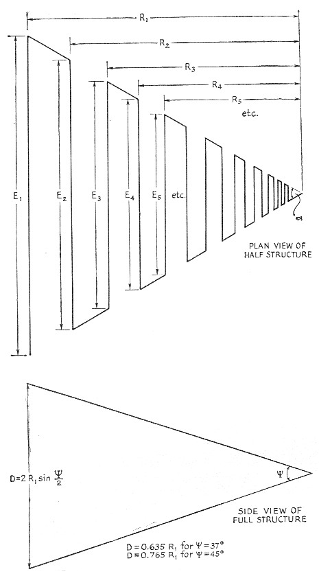
Fig. 2. Design dimensions of the log periodic antenna.
Now let's see what will be required to design and construct such an antenna.
Finding dimensions
As a point of departure, first let's decide on the lowest frequency on which we desire to operate. For instance, we may choose 14 Mc and want to operate up through 144 Mc. In this type of antenna the longest element, E1, is about,0.5 wavelength at lowest frequency selected. For 14 Mc we will use a figure of about 35 feet. On the logical basis that what is good enough for the experienced designer should be good enough for us, we will use the published design factors used by DuHamel for his Collins Model 237A series. He picked an apex angle, a, of 60 degrees in the horizontal plane for each half of the antenna. A vertical angle, ψ, of 37 degrees between the two half structures was chosen to provide a 90 degree vertical pattern. A periodic function τ of 0.6 was arbitrarily selected. The gain for this design is about 6 db. over a dipole and an azimuth beam pattern of about 65 degrees is obtained.
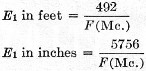
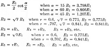
The second step is to determine the distance R1 from the apex (feed point) to the center of the longest element. From our high school geometry we can determine that this is about 30.3 feet, using the equations for right triangles, since we know all the angles and the length of one triangle side is half the chosen longest element's length. The equation I used was
![]()
which, since a = 60°, is 0.866E1 or 30.3 feet.
Next we obtain the position of the third element by multiplying this Rl by the r of 0.6 and get 18.2 feet for R3. Now what about the second element? From DuHamel's equations this will be R2 = R1-Vr, so when r = 0.6, R2 = 0.775R1. As you can see, this is actually the geometric mean between R1 and R3. Multiplying this out we get 23.5 feet for the second-element spacing, The rest is easy, for we need only multi. ply by r to get the values R4 = 0.6R2-R5 = 0.6R3, and so on. The identical procedure will yield the element lengths since they have the same periodic relationship.
The tables show values for construction of various practical antennas. Tables I and II are for 20 meter and up, Table III is for 10 meter and up, and Table IV is a v.h.f. man's dream. It covers continuously from 50 Mc through the TV, f.m., aircraft and satellite bands, 144, 220 and 450 Mc, all in one structure having 6 dB gain - and which is only about the size of a good v.h.f. TV antenna.
| E1 = 35 foot α = 60° ψ = 37° τ = 0.6 D = 19' 3" Vertical pattern about 90° Azimuth pattern about 65° Gain about 6 dB over dipole | |
| E1 = 35' 0" | R1 = 30' 4" |
| E2 = 27' 2" | R2 = 23' 6" |
| E3 = 21' 0" | R3 = 18' 2" |
| E4 = 16' 3" | R4 = 14' 1" |
| E5 = 12' 8" | R5 = 10' 11" |
| E6 = 9' 9" | R6 = 8' 6" |
| E7 = 7' 7" | R7 = 6' 6" |
| Es = 5' 10" | R8 = 5' 1" |
| E9 = 4' 7" | R9 = 3' 11" |
| E10 = 3' 6" | R10 = 3' 0" |
| E11 = 2' 9" | R11 = 2' 4" |
| E12 = 2' 2" | R12 = 1' 10" |
| E13 = 1' 8" | R13 = 1' 5" |
| E14 = 1' 3" | R14 = 1' 1" |
| Eis = 1' 0" | R15 = 0' 10" |
| E16 = 0' 9" | R16 = 0' 8" |
| E1 = 35 feet α = 45° ψ = 45° D = 32'5" τ either 0.6 or 0.707 Vertical pattern about 66° Azimuth pattern about 66° Gain about 7.7 dB over dipole | |||
| Dimensions when τ = 0.6 | Dimensions when τ = 0.707 | ||
| E1 = 35' 0" | R1 = 42' 3" | E1 = 35' 0" | R1 = 42' 3" |
| E2 = 27' 2" | R2 = 32' 9" | E2 = 29' 5" | R2 = 35' 6" |
| E3 = 21' 0" | R3 = 25' 4" | E3 = 24' 9" | R3 = 29' 10" |
| E4 = 16' 3" | R4 = 19' 8" | E4 = 20' 9" | R4 = 25' 2" |
| E5 = 12' 8" | R5= 15' 3" | E5 = 17' 6" | R5 = 21' 2" |
| E6 = 9' 9" | R6 = 11' 9" | E6 = 14' 9" | R6 = 17' 9" |
| E7 = 7' 7" | R7 = 9' 2" | E7 = 12' 4" | R7 = 15' 0" |
| E8 = 5' 10" | R8 = 7' 1" | E8 = 10' 5" | R8 = 12' 7" |
| E9 = 4' 6" | R9 = 5' 6" | E9 = 8' 9" | R9 = 10' 7" |
| E10 = 3' 6" | R10 = 4'3" | E10 = 7' 4" | R10 = 8' 10" |
| E11 = 2' 9" | R11 = 3' 4" | E11 = 6' 2" | R11 = 7' 6" |
| E12 = 2' 2" | R12 = 2' 6" | E12 = 5' 2" | R12 = 6' 3" |
| E13 = 1' 8" | R13 = 2' 0" | E13 = 4' 4" | R13 = 5' 4" |
| E54 = 1' 3" | R14 = 1' 6" | E14 = 3' 8" | R14 = 4' 5" |
| E15 = 1' 0" | R15 = 1' 2" | 15 = 3' 1" | R15 = 3' 9" |
| E16 = 0' 9" | R16 = 0' 11" | E16 = 2' 7" | R16 = 3' 2" |
| E17 = 2' 2" | R17 = 2' 8" | ||
| E18 = 1' 10" | R18 = 2' 3" | ||
| E19 = 1' 6" | R19 = 1' 10" | ||
| E20 = 1' 3" | R20 = 1' 7" | ||
| E21 = 1' 1" | R21 = 1, 4" | ||
| E22 = 0' 11" | R22= 1'2" | ||
| E23 = 0' 9" | R23 = 0' 11" | ||
| E1 = 17.7 feet α = 60° ψ = 37° τ = 0.6 D = 9'9" Vertical pattern about 90° Azimuth pattern about 65° Gain about 6 dB over dipole | |
| E1 = 17' 9" | R1 = 15' 4" |
| E2 = 13' 9" | R2 = 11' 11" |
| E3 = 10' 8" | R3 = 9' 3" |
| E4 = 8' 3" | R4 = 7' 2" |
| E5 = 6' 4" | R5 = 5' 6" |
| E6 = 4' 11" | R6 = 4' 3" |
| E7 = 3' 10" | R7 = 3' 4" |
| E8 = 3' 0" | R8 = 2' 7" |
| E9 = 2' 4" | R9 = 2' 0" |
| E10 = 1' 9" | R10 = 1' 6" |
| E11 = 1' 5" | R11 = 1' 2" |
| E12 = 1' 1" | R12 = 0'11" |
| El3 = 0' 10" | R13 = 0' 9" |
| E1 = 10 feet α = 60° ψ = 37° τ = 0.707 D = 5' 6" Vertical pattern about 90° Azimuth pattern about 65° Gain about 6 db. over dipole | |
| E1 = 10' 0" | R1 = 8' 8" |
| E2 = 8' 5" | R2 = 7' 3" |
| E3 = 7' 1" | R3 = 6' 2" |
| E4 = 6' 0" | R4 = 5' 2" |
| E5 = 5' 0" | R5 = 4' 4" |
| E6 = 4' 3" | R6 = 3' 8" |
| E7 = 3' 6" | R7 = 3' 1" |
| E8 = 3' 0" | R8 = 2' 7" |
| E9 = 2' 6" | R9 = 2' 2" |
| E10 = 2' 2" | R10 = 1' 10" |
| E11 = 1' 9" | R11 = 1' 6" |
| E12 = 1'6" | R12 = 1' 3" |
| E13 = 1' 3" | R13 = 1' 1" |
| E14 = 1' 0" | R14 = 0' 11" |
| Ei5 = 0' 10" | R15 = 0' 9" |
| E16 = 0' 9" | R16 = 0' 8" |
| E17 = 0' 8" | R17 = 0' 6" |
One important point to remember is that this antenna radiates forward from the longest element toward the feed point, unlike a conical or horn which it somewhat resembles in appearance.
Now that we have determined the dimensions, all that remains is to construct the working unit.
Building one
While it is possible to build the 14 Mc and-up unit as a rotary beam, as Collins does in their 237A series, it will be much simpler and less expensive to build a fixed array in the following manner:
Determine desired beam direction and put up a 15-foot vertical length of TV mast to support the apex or feed point. Next, set up two 30 foot TV type telescopic masts (about $7.50 each, locally) to support the ends of the rear longest elements. Their spacing will be about 40 feet or so on a horizontal line perpendicular to the end of a radius R1 drawn from the apex it; the direction opposite to the desired main lobe's bearing. Roughly, the three masts will form an equilateral triangle with the 15 footer at the apex located in the desired direction of radiation. The 65 degree wide main lobe should provide a satisfactory coverage area.
Now, by using stranded or, preferably, copper-weld antenna wire for elements and a quantity of polyethylene line for support, it should be easy to arrange the necessary radiating elements as determined by our calculated dimensions. The angle between the upper half-structure and the lower one will be about 37 degrees if we follow Collins' example, giving a separation of 19.2 feet between the open ends of the two halves of the antenna. The lower element should be arranged to be high enough off the ground so it will not be a hazard to persons.
A wire or boom should be used to connect all the centers of the elements of each half together. As this is a nodal balance point, it can be grounded for lightning protection. The best method of feeding may be to use a piece of tubing for the lower-half center bonding element and use it as a sleeve through which a coax line (RG-59/U or RG-11/13) can be passed. This will make it unnecessary to use any other type of line-balancing device. This feed coax will go from the rear to the apex feed point, where the coax shield will connect to the end of the shortest element of the lower half-structure and the center conductor will connect to the end of the shortest element of the top half-structure. Note that the upper and lower structures are opposite symmetrical structures and are not mirror images. This entire antenna should not cost over $35.00 to construct, exclusive of the feed line.
An experimental V.H.F. model
An antenna using the dimensions of Table IV was constructed for the purpose of getting some performance data on the system. At the time, the only available material was some brass tubing, and the resulting structure was much too heavy for one-man installation on a regular tower, so the tests were made at a height of about 12 feet. Using RG-59/U line to feed the antenna, s.w.r. measurements yielded the following data:
| Frequency (Mc) | S.W.R. in 75 Ω line |
|---|---|
| 50.04 | 1.4 to 1 |
| 50.4 | 1.45 to 1 |
| 51.25 | 1.5 to 1 |
| 144.12 | 1.05 to 1 |
| 144.72 | 1.5 to 1 |
| 144.9 | 1.7 to 1 |
| 145.35 | 2.1 to 1 |
| 145.8 | 1.9 to 1 |
| 146.25 | 1.6 to 1 |
| 146.7 | 1.1 to 1 |
| 147.12 | 1.2 to 1 |
| 147.6 | 1.5 to 1 |
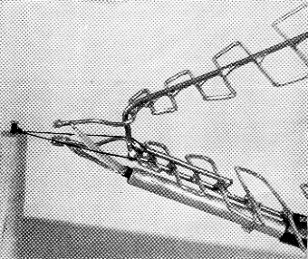
Fig. 3. Feed arrangement using coaxial cable. There is a voltage node at the center of each element, so a metallic support may be bonded to the centers without disturbing the operation of the antenna. The coax is run through a sleeve fastened to the support for the lower half-structure, thereby decoupling the coax shield from the antenna.
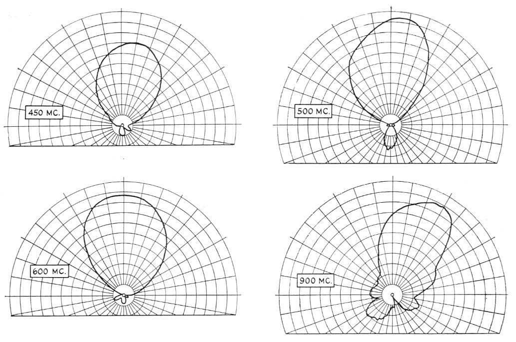
Fig. 4. Measured patterns of the u.h.f. model shown in Fig. 1, at four frequencies between 450 and 900 Mc.
Similar checks were made with 52 ohm RG-58/U feed line, and comparison of the standing-wave ratios with those observed for RG-59/U indicated that the impedance of the antenna is actually greater than 75 ohms. The feed line I would recommend is 95 ohm RG-62/U, which has much lower loss than either RG-58/U or RG-59/U but costs only about $6 per hundred feet. RG-63/U (125 ohms) might provide even a better match, but costs about twice as much.
Although the experimental antenna was tried only at the 12 foot height, it provided a number of 6 and 2 meter contacts with various points in Connecticut, using Communicators. On TV reception it gave excellent performance as compared with a Channel-Master Super-Rainbow which was at a height of 45 feet, and on the f.m. band it out-performed the TV antenna despite the difference in height. A similar antenna, using lighter construction so the weight will be manageable, is planned for the near future.
Other configurations
All this is fine, you say, but these gain figures are a bit low compared with what is claimed for some one-band arrays, so how can we "hot rod" it to get higher gain? First, it is not practical to stack antennas because stacking will introduce a frequency-dependent factor. There are several methods for getting moderate improvements at the expense of beam coverage or increasing the number and size of elements.
One method which will provide up to 10.5 dB gain is to decrease the apex angle, a, and increase the periodic function, τ. An angle of 45 degrees with a τ of 0.707 and a separation angle of 45 degrees will give us 7.7 dB gain with little change in azimuth pattern and an acceptable decrease of vertical coverage to 66 degrees. The length from apex to rear element grows from about 30 feet to about 42 feet (Table II) and the total number of elements increases slightly. Changing the apex angle to 15 degrees will permit 10.5 db. gain, but the antenna will become much longer and the number of elements will be considerably greater. As always, you do not get something for nothing. The azimuth beam width does not drop too much, being in the order of 57 degrees as compared with 65 degrees.
Another method is to interlace four half-structures with the same apex point, with each pair having a different spacing angle. Another is to build two identical units side by side with the same apex feed point. The problem here is proper phasing of elements, as improper connection can produce a twin-lobed difference pattern.
One of these antennas aimed vertically with the apex at top of a mast, using the elements as the guy structure, should be a natural for satellite work, as it could operate on 20, 40, or 108 Mc., and any other future frequencies in between, and have the same gain and beam pattern for any of the frequencies. A gain of 10 db. or more could be secured, and by arranging the antennas in the form of a pyramid the two sets of elements could be phased either to produce a sum pattern with one main lobe or a difference pattern with a null directly overhead, like a doughnut with the hole at the apex feed point. The feed coax in this case could be fed up through the support mast.
It seems time that we amateurs take notice of the excellent characteristics of this antenna design and put it to use. How about you? The writer will be most interested to hear of the results from anyone who tries it out, and R. H. DuHamel, the originator, will undoubtedly be interested, also.
Appendix I
Definitions
E1 = length of longest element approximatley (λ/2 at lowest operating frequency).
R1 = distance from apex to center of E1, the longest element.
E2 = length of second longest element.
R2 = distance from apex to center of E.
τ = periodic function.
α = apex angle or horizontal angle made by radials from apex to ends of elements.
ψ = apex angle or vertical separation angle between the two half-structures.
Appendix II
Design equations
Notes
- Space Aeronautics Magazine, March, 1959, p. 148. 1958 IRE Convention Record, Part 1, p. 139. 1958 IRE WES-CON Convention Record, Part 1. 1957 IRE Convention Record, Part 1, p. 119.
Carl T. Milner, W1FVY.