Some amateur applications of the Smith chart
Simplifying transmission-line problems.
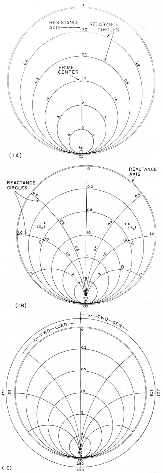
Fig. 1. Construction of the Smith Chart.
A Resistance scales.
B Chart with reactance scales added.
C Wavelength scales.
One of the most useful tools at the disposal of the radio engineer is a transmission-line calculator known as the Smith Chart. This device eliminates the need for mathematical gymnastics and greatly reduces the laborious task of solving most transmission-line problems. In this article, K6CRT discusses the use of the Chart in some of its simpler applications.
In All probability, the chief reason that more use of the Smith Chart is not made by amateurs in solving some of their antenna-feeding problems is its formidable appearance at first glance. But a brief description of its construction and some of its simpler applications will show that it is far less complicated than its aspect.
Resistance scales
Referring to Fig. 1, the Smith Chart(1) consists basically of a circle upon which are placed various circular scales. The only straight line on the Chart - the vertical one in Fig. 1A - is the resistance axis. The numbers along this line indicate percentages of the value assigned to the center point - the 100 per cent point indicated by the numeral 1.0 - usually referred to as prime center. The calibration of this line runs from 0 at the top to infinity (∞) at the bottom. If prime center is assigned a value of 100 ohm, then 0.5 represents 50 ohm, 0.2 represents 20 ohm, 2.0 represents 200 ohm, etc. If a value of 50 ohm is assigned to prime center, corresponding values will be 25, 10 and 100 ohm.
It is seen that in each case the point on the Chart for any resistance value is determined by dividing the value by the number assigned to prime center. This is called "normalizing." Similarly, points on the Chart are converted back to actual resistance values by multiplying by the value assigned prime center. This process permits the use of the numbers printed on the Smith Charts for values irrespective of their magnitudes. It is common practice to indicate actual impedance values in capital letters (Z1, ZA, ZL, etc.) and corresponding normalized values in small letters (z1, zA, zL, etc.).
Resistance circles (see Fig. 1A) are centered on the resistance axis, are tangent to the outer circle at the R = ∞ point, and pass through the calibrated points on the resistance axis. All points along any resistance circle have the same resistive value as the point where the circle crosses the resistance axis.
Reactance scales
Superimposed on the resistance-circle pattern are segments of other circles tangent to the resistance axis at R = ∞. See Fig. 1B. These are reactance circles, the large outer circle being the reactance axis. The reactance axis is also calibrated in percentages of a selected value - usually the value assigned to prime center. All points along any reactance circle have the same reactive value as the point where the reactance circle touches the reactance axis (outer circle). Values to the right of the resistance axis are positive (inductive), and those to the left of the resistance axis are negative (capacitive).
Plotting Impedances
The plotting of complex impedances can best be explained by one or two examples. Suppose we have an impedance consisting of 50 ohm resistance and 100 ohm inductive reactance (Z = 50 + j100). If we assign a value of 100 ohm to prime center (Z0 = 100), the z point will be plotted at the intersection of the 50/100 = 0.5 resistance circle and the 100/100 = 1.0 positive reactance circle (point A in Fig. 1B). If a value of 50 ohm had been assigned to prime center, the same impedance would be plotted at the intersection of the 50/50 = 1.0 resistance circle and the 100/50 = 2.0 reactance circle (point B in Fig. 1B).
For example, if a value of 200 is assigned to prime center, then point C in Fig. 1B represents an impedance of 0.5 × 200 = 100 ohm resistance, and 1.0 × 200 = 200 ohm negative (capacitive) reactance (Z = 100 - j200).
In solving transmission-line problems, prime center is usually assigned a value equal to the characteristic impedance of the transmission line to be used. Always record this value at the start to avoid any possible confusion later on.
Wavelength scales
Aside from the calibrations already mentioned, the perimeter of the large circle has additional scales. Two of these scales (see Fig. 1C) are calibrated in terms of portions of a wavelength along a transmission line, one scale (running counterclockwise) starts at the generator (transmitter) end of the line and progresses toward the load (antenna), while the other scale, in reverse, starts at the load and works back toward the generator. The complete circle represents a half wavelength. It is assumed that no amateur should have difficulty in determining portions of an electrical wavelength from the formula:
![]()
where l = length in ft. and k is the velocity factor furnished in transmission-line characteristic tables. Since the same conditions repeat every half wavelength along the line, the zero point on the wavelength scales may be considered as any multiple of a half wavelength as well as zero. The use of the wavelength scales will be illustrated presently.
Impedance transformation
When a lossless transmission line is terminated in some impedance other than a pure resistance having a magnitude equal to the characteristic impedance of the line, the input impedance of the line will vary depending on the length of the line. If the terminating impedance is known, it is a simple matter to determine the input impedance of the line for any length of line by means of the Smith Chart.
First we plot the load (antenna) impedance on the Chart. Suppose we have an antenna that shows a resistive component of 25 ohm and an inductive reactance of 25 ohm (ZA = 25 + j25). If the transmission line has a characteristic impedance of 50 ohm, we normalize the antenna impedance by dividing by 50 (zA = 0.5 + j0.5). This is plotted as point zA on the Chart of Fig. 2.
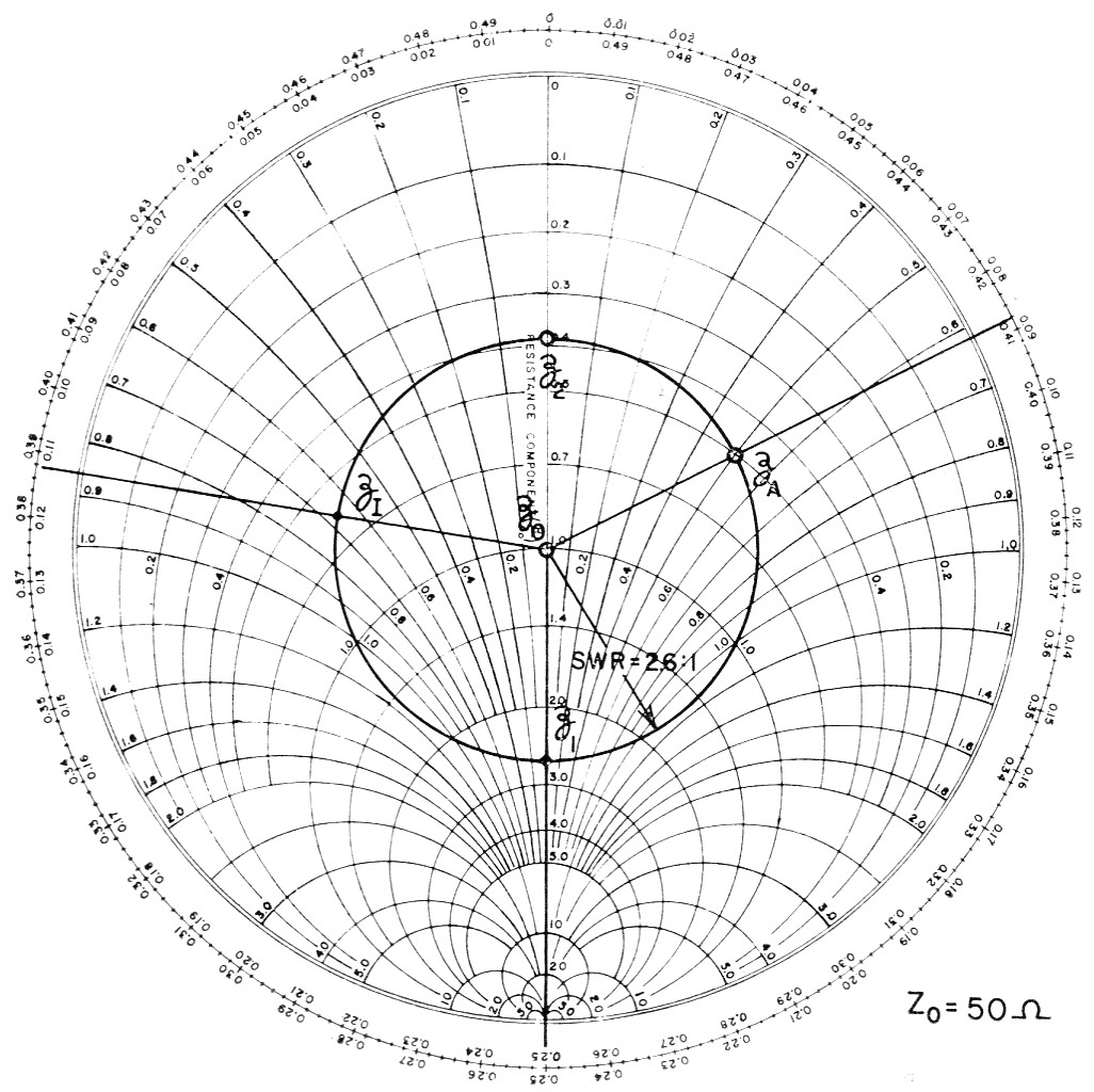
Fig. 2. Determining line input impedance (Zi) when antenna impedance (ZA) and line length are known. At two line lengths, the input impedance will be resisve and have values (normalized) of z1 and z2.
A circle whose center is on prime center and whose perimeter passes through the plotted point is next inscribed on the Chart. This circle is usually referred to as an s.w.r. circle, since the s.w.r. on the line when terminated by the plotted impedance can be determined by the points at which the circle crosses the resistance axis. The s.w.r. (2.6 in this case) may be read directly where the bottom of the circle crosses the resistance axis. (The reading of 0.384 at the top of the circle is the reciprocal - 1/2.6 - which, of course, indicates the same s.w.r.)
The next step in determining the input impedance of the line is to draw a vector from prime center through zA to intersect the wavelength scales. Since we are starting at the load, the "Toward Generator" scale is used. To find the input impedance of the line at any desired distance from the antenna, we simply rotate the vector through this distance along the wavelength scale. The zA vector intersects the wavelength scale at 0.088. If we want to find the line input impedance when the line is 0.3 wavelength long, for instance, we add 0.088 + 0.3 = 0.388 and move the vector to this point on the wavelength scale. Then the normalized impedance is read at the intersection of the new vector and the s.w.r. circle. The reading here is zi = 0.6 - j0.67. The actual input impedance is obtained by multiplying back by the line Z0 = 50, to give Z1 = 30 - j33.5 (30 ohm resistance, 33.5 ohm capacitive reactance).
It is interesting to note that the Chart indicates two line lengths for which the input impedance will be resistive. These points are indicated by z1 and z2 in Fig. 2, where the antenna-impedance vector swings across the resistance axis. One of these lengths is 0.25 - 0.088 = 0.162 wavelength; the other is 0.5 - 0.088 = 0.412 wavelength. Since the Chart reading at zi is 2.6, j0, the line input impedance ZI = 50 × 2.6 = 130 ohm for the 0.162-wavelength line. Similarly, the reading at zi is 0.384, j0 and the input impedance with the 0.412-wavelength line is 50 × 0.384 = 19.2 ohm. It should always be remembered that any number of half wavelengths can be added to the lengths given by the Chart without changing the line input impedance (assuming a lossless line). From this, it can be seen that a transmission line terminated in a load not the same as the characteristic impedance of the line acts as an impedance transformer, transforming the value of the load resistance to some other value at the input to the line. By proper selection of line length characteristic impedance, any load resistance can be transformed to any other value desired.
Measuring antenna impedance remotely
From the foregoing, it may be evident that the process can be reversed to determine the feed-point impedance of the antenna when the length of the line and the line input impedance are known. The line input impedance can be measured by means of an impedance bridge. The electrical length can also be determined either by direct measurement of its physical length and applying the velocity factor, or indirectly by measuring the input impedance of the line when the line is terminated in a short circuit.
In one actual measurement made by the author, the input impedance of a 50 ohm line terminated in a short circuit was 2.5 + j50, or a normalized value of 0.05 + j1. This point, zis, is shown plotted on a Smith Chart in Fig. 3. The terminating load in this case is ZLS = 0 + j0 (a short circuit). The vector for this load coincides with the upper half of the resistance axis. Using the "Toward Generator" scale, we find that the distance between the ZLS vector and the ZLS vector is 0.125 wavelength. This is the electrical length of the line.
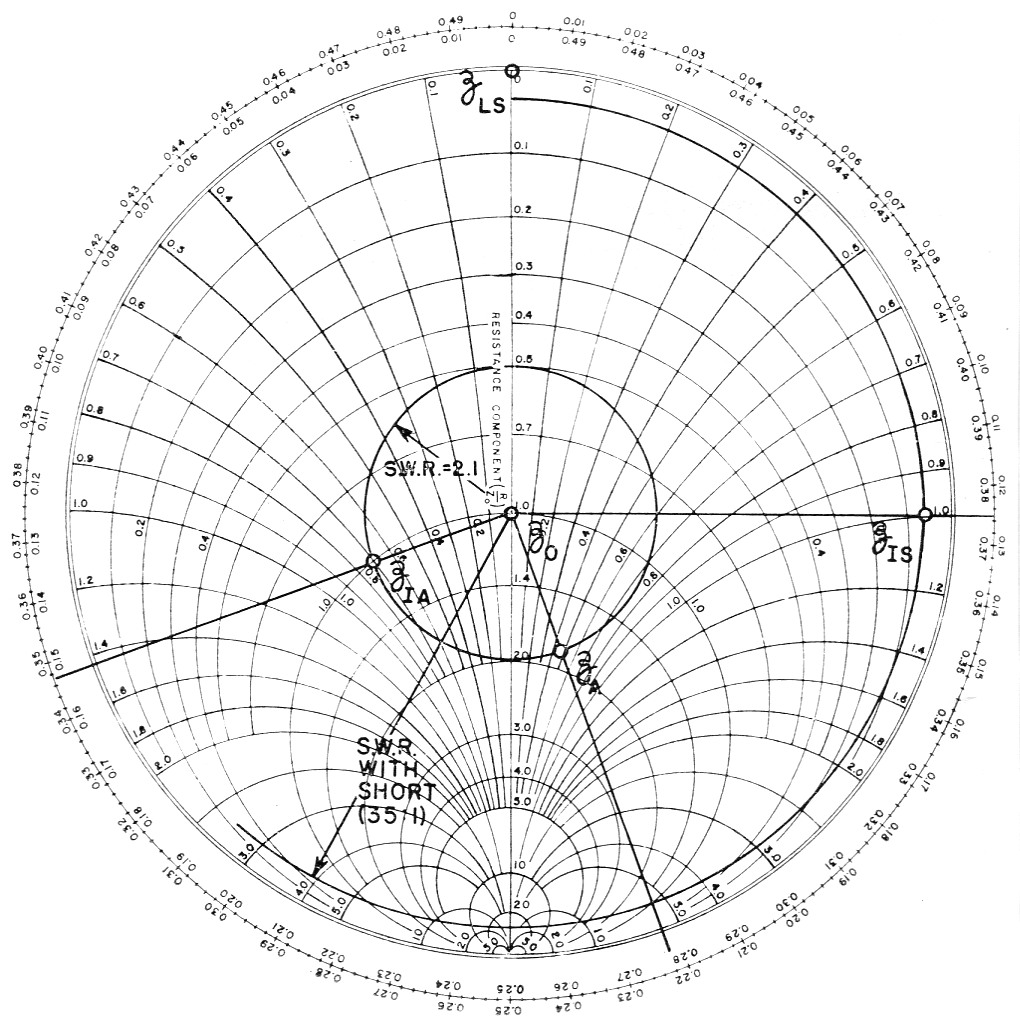
Fig. 3. Chart for determining antenna impedance (ZA) from measured line input impedances, ZIA with line terminated in an antenna, ZLS with the line terminated in a short circuit.
With the antenna replacing the short circuit, the line input impedance was measured at ZIA = 50 - j35, which normalizes to zIA = 1.0 - j0.7. This impedance is plotted, the s.w.r. circle is scribed and the ZIA vector drawn. Since this is the line input impedance, the "Toward Load" scale is used. The vector intersects the wavelength scale at 0.153. The vector is now moved the length of the transmission line - 0.125 wavelength - toward the load, to 0.153 + 0.125 = 0.278 wavelength. The normalized antenna impedance, zA, can now be read at the intersection of the new vector and the s.w.r. circle. The Chart shows this value to be 1.82 + j0.48, which gives an actual value of ZA = 50 (1.82 + j0.48 = 91 + j24. The s.w.r. circle shows that the s.w.r. on the line is 2:1.
Cable attenuation
In the foregoing, a lossless transmission line has been assumed. With a practical line, the s.w.r. will change with the length of the line, being greatest at the load end of the line and decreasing as the length of the line is increased. Similarly, losses in the transmission line will cause the line input impedance to vary as the length of the line is changed, even though the line may be terminated in an accurately-matched load. Therefore, s.w.r. measurements made at the input end of the line are not a strictly true indication of the mismatch between the load and the transmission line, and losses in the line will cause some error in the calculations of load impedance from measurements of impedance made at the input to the line, unless suitable correction is applied. The error in both cases will be small if the line is short and has low inherent loss, and the load is reasonably well matched to the line. The error will be greater if the line is long, has high loss per unit length, or if it is operated at a high s.w.r.
True values of s.w.r. and load impedance can be determined from the Smith Chart if the total line loss is known, as in the following example.
The input impedance of a 50 ohm terminated line having a loss of 3 dB is measured and found to be ZIM = 100 + j0. This measured value is normalized and plotted and the s.w.r. circle and vector are drawn as shown in Fig. 4. The chart of Fig. 5 shows that a line having a 3 dB loss when terminated by a load equal to the characteristic impedance of the line will have an s.w.r. of 3 when terminated in a short circuit. This s.w.r. circle is drawn on the chart. A line ABC is drawn at right angles to the zus vector, intersecting the s.w.r. circle of the shorted line and the reactance axis. A straight line is then drawn from B to zIM. A second line parallel to the latter is drawn from point C to intersect the ZIA( vector. An s.w.r. circle drawn through this intersection indicates the true s.w.r. (4.8). (It should be noted that the ratio of measured load impedt ance, 100 + j0, to the line characteristic impedf ance, 50 ohm, would indicate an s.w.r. of only 2 to 1.) The true value of load impedance is 4.8Z0 = 4.8 × 50 = 240 ohm. (This compares with the measured value of 100 ohm.)
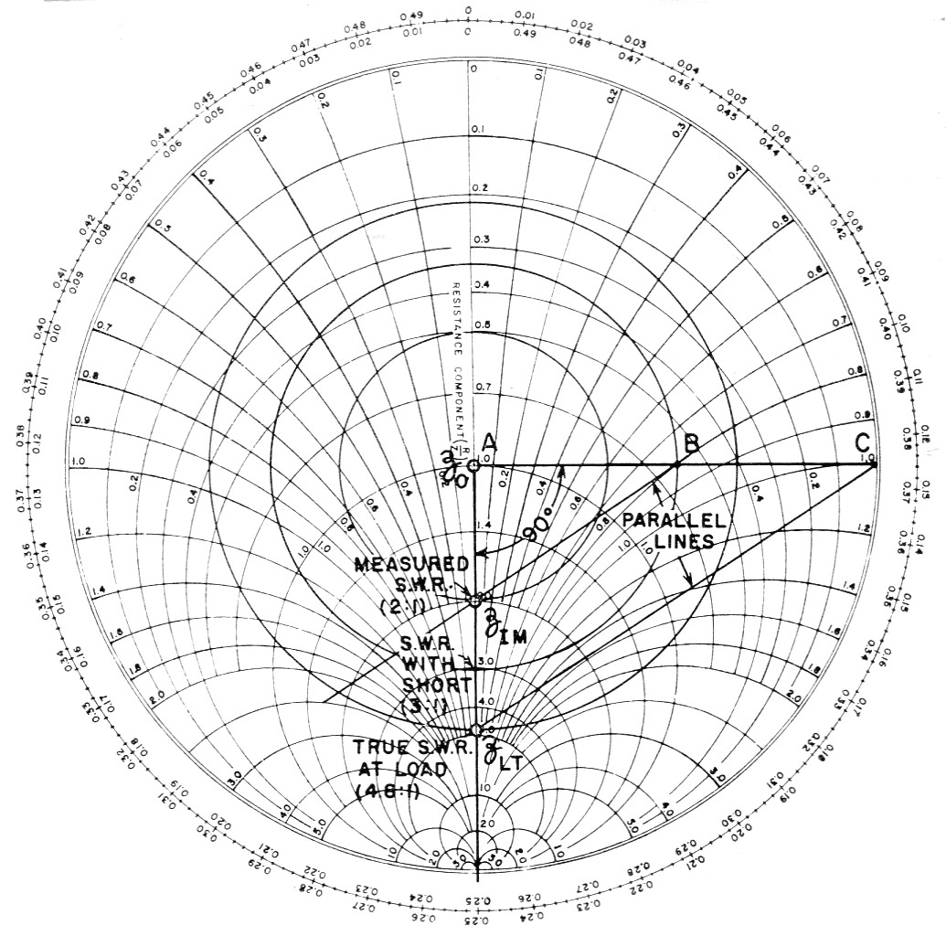
Fig. 4. Chart for correcting for losses in transmission line. ZIM is the measured input impedance of the line; ZLT is the true load impedance.
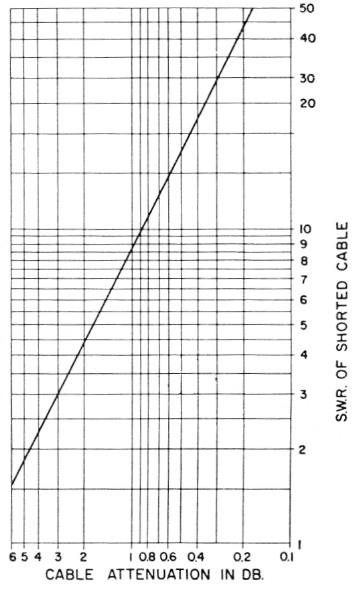
Fig. 5. Graph showing the relationship between the s.w.r. measured with a line terminated in a short circuit and the loss in dB measured when the line is terminated in its characteristic impedance.
The loss of 3 dB used in this example is representative of what might be found in a 150 foot length of small coax cable at 28 Mc. So the next time anyone tells you that his s.w.r. is 1 to 1, you will have good reason to doubt his accuracy.
If the same construction is applied to Fig. 3, it will be found that the true values will be only slightly different from the uncorrected values. In this case the s.w.r. with the line shorted is 35 to 1, corresponding to a line loss of 0.25 dB on the chart of Fig. 5. This low line loss, of course, accounts for the smaller error.
Notes
L.A. Cholewski, K6CRT, EX-W8SVK.