Noise factors affecting V.H.F. communication
Cosmic, receiver and transmission-line noise - All out to get your signal.
V.h.f. DXers are constantly fighting something even tougher than QRM - noise. The tables in this article will tell you what kind of noise is the limiting factor in your particular situation. The best and worst times of day for cosmic noise are also tabulated. Add to this the information on path attenuation and predicting signal-to-noise ratio, and you have must reading for every v.h.f. enthusiast.
V.H.F. amateur radio communication is limited by several factors not significant at h.f. These factors include scattering-type propagation, noise generated by the receiver and cosmic noise picked up by the antenna. This article will discuss the noise limitations and should help the amateur to minimize the noise in his receiving system.
Many v.h.f. men have noticed that connecting the antenna to a 6-meter receiver increases the noise output much more than if the same thing is done at 2 meters or above. This means that at 6 meters the noise coming down from the antenna system is more than that generated in a typical receiver; on higher frequencies, the converse is true.
The noise coming from the antenna may be thought of as having three components. One component is proportional to the temperature of and loss in the transmission line. The other two components are both generated far from the antenna system. One comes from radiation in the region of the center of the galaxy and will be called the galactic component. The other may be considered an average radiation from many extraterrestrial and upper atmosphere noise generators; this will be called the background component. Together, the galactic and background components make up what is often called cosmic noise.
The galactic component is stronger than the background component, and its source is much more localized in space. This means that an antenna pointing in a certain direction will be receiving only the relatively weak background component most of the time. However, at some time of day (for most bearings) the motion of the earth relative to the "fixed" galaxy will cause the stronger galactic noise source to pass through the antenna beam. When this occurs, the noise is at a maximum for the day, and v.h.f. communication is at its worst. Table I shows the time of day when noise input to the antenna is a maximum as a function of the month and the direction in which the antenna is pointing.
| Antenna heading | ||||||||
|---|---|---|---|---|---|---|---|---|
| Month | N | NE | E | SE | S | SW | W | NW |
| Jan. | - | 0330-0700 | 0500-0800 | 0630-1000 | 1000-1400 | 1300-1600 | 1500-1900 | 1800-2130 |
| Feb. | - | 0130-0500 | 0300-0600 | 0430-0800 | 0800-1200 | 1100-1400 | 1300-1700 | 1600-1930 |
| Mar. | - | 2330-0300 | 0100-0400 | 0230-0600 | 0600-1000 | 0900-1200 | 1100-1500 | 1400-1730 |
| Apr. | - | 2130-0100 | 2300-0200 | 0030-0400 | 0400-0800 | 0700-1000 | 0900-1300 | 1200-1530 |
| May | - | 1930-2300 | 2100-0000 | 2230-0200 | 0200-0600 | 0500-0800 | 0700-1100 | 1000-1330 |
| June | - | 1730-2100 | 1900-2200 | 2030-0000 | 0000-0400 | 0300-0600 | 0500-0900 | 0800-1130 |
| July | - | 1530-1900 | 1700-2000 | 1830-2200 | 2200-0200 | 0100-0400 | 0300-0700 | 0600-0930 |
| Aug. | - | 1330-1700 | 1500-1800 | 1630-2000 | 2000-0000 | 2300-0200 | 0100-0500 | 0400-0730 |
| Sep. | - | 1130-1500 | 1300-1600 | 1430-1800 | 1800-2200 | 2100-0000 | 2300-0300 | 0200-0530 |
| Oct. | - | 0930-1300 | 1100-1400 | 1230-1600 | 1600-2000 | 1900-2200 | 2100-0100 | 0000-0330 |
| Nov. | - | 0730-1100 | 0900-1200 | 1030-1400 | 1400-1800 | 1700-2000 | 1900-2300 | 2200-0130 |
| Dec. | - | 0530-0900 | 0700-1000 | 0830-1200 | 1200-1600 | 1500-1800 | 1700-2100 | 2000-2330 |
Times are given in EST; they can be converted in the usual way for use in other time zones. These times are for the United States and will be different for places with other latitudes. For mid-latitudes in the United States the maximum noise source never passes across the northern horizon. Hence no times are given.
The background component is not really uniform, since there are regions which are radiating less than other regions. Therefore, times of the day when the noise is at a minimum also exist. Table II indicates when they are.
| Antenna Heading | ||||||||
|---|---|---|---|---|---|---|---|---|
| Month | N | NE | E | SE | S | SW | W | NW |
| Jan. | 1030-1430 | 1530-1930 | 1830-2200 | 2130-0000 | 0000-0300 2000-2230 | 0300-0545 | 0530-0730 | 0630-1000 |
| Feb. | 0830-1230 | 1330-1730 | 1630-2000 | 1930-2200 | 1800-2030 2200-0100 | 0100-0345 | 0330-0530 | 0430-0800 |
| Mar. | 0630-1030 | 1130-1530 | 1430-1800 | 1730-2000 | 1600-1830 2000-2300 | 2300-0145 | 0130-0330 | 0230-0600 |
| Apr. | 0430-0830 | 0930-1330 | 1230-1600 | 1530-1800 | 1400-1630 1800-2100 | 2100-2345 | 2330-0130 | 0030-0400 |
| May | 0230-0630 | 0730-1130 | 1030-1400 | 1330-1600 | 1200-1430 1600-1900 | 1900-2145 | 2130-2330 | 2230-0200 |
| June | 0030-0430 | 0530-0930 | 0830-1200 | 1130-1400 | 1000-1230 1400-1700 | 1700-1945 | 1930-2130 | 2030-0000 |
| July | 2230-0230 | 0330-0730 | 0630-1000 | 0930-1200 | 0800-1030 1200-1500 | 1500-1745 | 1730-1930 | 1830-2200 |
| Aug. | 2030-0030 | 0130-0530 | 0430-0800 | 0730-1000 | 0600-0830 1000-1300 | 1300-1545 | 1530-1730 | 1630-2000 |
| Sept. | 1830-2230 | 2330-0330 | 0230-0600 | 0530-0800 | 0400-0630 0800-1100 | 1100-1345 | 1330-1530 | 1430-1800 |
| Oct. | 1630-2030 | 2130-0130 | 0030-0400 | 0330-0600 | 0200-0430 0600-0900 | 0900-1145 | 1130-1330 | 1230-1600 |
| Nov. | 1430-1830 | 1930-2330 | 2230-0200 | 0130-0400 | 0000-0230 0400-0700 | 0700-0945 | 0930-1130 | 1030-1400 |
| Dec. | 1230-1630 | 1730-2130 | 2030-0000 | 2330-0200 | 0200-0500 2200-0030 | 0500-0745 | 0730-0930 | 0830-1200 |
Both galactic and background components behave the same in that their strengths fall off rapidly with an increase in frequency. Doubling the frequency will decrease the cosmic noise some 5.8 times, so at 144 Mc. the background has shrunk to a small fraction of its value at 50 Mc. Table III gives the noise power density of the extraterrestrial components as a function of frequency. Note that the units used are watts per c.p.s. Multiplying these values by the bandwidth of the receiver in c.p.s. gives the noise power contribution in watts × 10-21.
| Cosmic noise power density (10-21 Watt/C.P.S.) | |||
|---|---|---|---|
| Frequency (Mc.) | Average | Maximum | Minimum |
| 50 | 84 | 248 | 50 |
| 144 | 3.7 | 9.5 | 3.3 |
| 220 | 2.1 | 6.6 | 1.2 |
| 430 | 0.4 | 1.2 | - |
Table IV gives the noise contributed by the transmission line as a function of line loss. Since line losses increase with frequency, so does this component of noise. An average temperature of -63 degrees F is assumed. In winter, with a cold transmission line, these values may be some 10 per cent less.
| Loss (dB)) | N.P.D. (10-21 Watt/C.P.S.) |
|---|---|
| 0.1 | .09 |
| 0.2 | .18 |
| 0.3 | .27 |
| 0.4 | .35 |
| 0.5 | .44 |
| 0.6 | .52 |
| 0.7 | .60 |
| 0.8 | .67 |
| 0.9 | .75 |
| 1.0 | .82 |
| 2.0 | 1.48 |
| 3.0 | 2.00 |
Table V converts receiver noise figure to the units given in Tables III and IV. Using typical values for noise figure and transmission-line loss it is easy to see that cosmic noise is the limiting noise factor at 6 meters. At 2 meters, on the other hand, receiver noise becomes very important as does, in many cases, noise from the transmission line.
| Receiver Noise Figure (dB) | Equivalent noise power density (10-21 Watts/C.P.S.) |
|---|---|
| 2 | 2.34 |
| 3 | 3.98 |
| 4 | 6.05 |
Summing the contributions from Tables III, IV and V will give the noise power which must be overcome by the signal. Then with a knowledge of the path attenuation, transmitter power and receiving and transmitting antenna gains it is possible to make a good estimate of the signal-to-noise ratio of a circuit.
Fig. 1 is presented to give the amateur some idea of the path attenuation he may encounter. Of course, many amateurs are not separated by smooth earth, and some stations have antennas more than 30 feet above the ground. To calculate path attenuation for these more general cases, some additional reading(1) will be required.
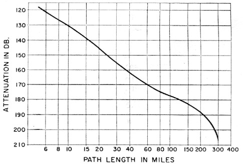
Fig. 1. Path attenuation as a function of the distance between two isotropic (same field in all directions) antennas 30 feet above ground and separated by smooth terrain. The curve shown is good for 6 and 2 meter.
Consider two 6-meter stations that are separated by smooth ground and have 30-foot high antennas. The rest of the circuit specifications are as follows:
| Distance between stations | 250 miles |
| Transmitting antenna gain | 9.0 dB over dipole |
| Line loss | 0.3 dB |
| Receiving antenna gain | 12.1 dB over dipole |
| Line loss | 1.0 dB |
| Receiver noise figure | 4 dB |
| Receiver bandwidth | 3000 c.p.s. |
| Transmitter power output | 250 watt |
First, find and total the noise contributions. From Table III the average cosmic noise power density at 50 Mc is 84 × 10-21 watt/c.p.s. The 1.0 dB receiving transmission-line loss converts to 0.82 × 10⁻²¹ watt/c.p.s. with the aid of Table IV. Table V says that a receiver noise figure of 4 dB is equivalent to a noise power density of 6.05 × 10⁻²¹ watt/c.p.s. Adding these three figures gives 90.87 × 10⁻²¹ watt/c.p.s., and multiplying this times the receiver bandwidth yields 2.73 × 10⁻¹⁶ watt as the noise power at the receiver.
Next, figure the net path attenuation from. transmitter to receiver. There are three losses involved: path -194 dB from Fig. 1, transmitting transmission line -0.3 dB, and receiving transmission line -1.0 dB. The gains are those of the transmitting antenna 9.0 + 2.2 (2.2 dB is the gain of a dipole over an isotropic radiator) dB, and the receiving antenna 12.1 + 2.2 dB Adding up the losses and the gains and subtracting the gains from the losses gives a net path attenuation of 169.8 dB.
Now the transmitter output power must be reduced by the path attenuation to get the signal power at the receiver.
Solving,
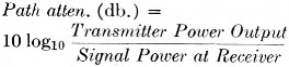
gives 2.61 × 10⁻¹⁵ watt as the signal power at the receiver. The signal-to-noise ratio equals this figure divided by the noise power at the receiver. Therefore,
![]()
A major portion of the information given in this paper was derived from Celestial Radio Radiation by Drs. J. D. Kraus and H. C. Ko, published by the Radio Observatory, Dept. of Electrical Engineering, Ohio State University. This work was done while the authors were research assistants at the National Radio Astronomy Observatory.(2) The authors wish to express their appreciation for the encouragement of Dr. John W. Findlay, Chairman of the Research Equipment Development Department and Assistant to the Director at the National Radio Astronomy Observatory.
Notes
- See the October 1955 issue of the Proceedings of the IRE, in particular, page 1488. Also, National Bureau of Standards Technical Notes No. 15, Prediction of the Cumulative Distribution with Time of Ground Wave and Tropospheric Wave Transmission Loss, Part I - The Prediction Formula; and No. 12, Transmission Loss in Radio Propagation II. These last are available for $1.50 and $3.00, respectively, from the Office of Technical Services, U. S. Department of Commerce, Washington 25, D. C.
- Operated by the Associated Universities, Inc., under contract with the National Science Foundation.
James C. McLaughlin, W8TBZ
Robert W. Hobss, W8PIL.