A method for determining V.H.F. station capabilities
Using readily obtainable data to plot reliable range.
If you have ever wondered about the maximum distance that could be worked by your v.h.f. station under normal propagation conditions, you probably decided that to determine the answer would be a sizable task. There is a great deal of literature on the subject, but much of it is too theoretical for the practical person. Then, even if an answer is obtained, you still may question whether it is just a theoretical number or the right answer.
After reading a recently published paper on ground wave and tropospheric scatter propagation,(1) I became interested to see if the answers that the theory predicted held true for an amateur radio station, where the antenna site and many other factors were not optimum. After running schedules over a period of months with K2GQI and W4LTU, I found that the measured signal strength checked with predicted signal levels within the limit of accuracy of my measuring equipment. Since the theory seemed to hold for amateur radio stations, other v.h.f. enthusiasts may be interested in having a relatively simple method of calculating the working range of their stations. Some might be surprised at how far they should be able to work. Such information is also useful to determine what station changes should be made to work a station that is presently just out of reach of reliable communications.
In order to make the calculation as straightforward as possible, data and graphs given by Norton have been reduced to nomogram form for the amateur frequencies from 50 to 1300 Mc. Before we get into the method of calculation, however, a few interesting things can be determined by plotting the path loss as a function of distance. The path loss is the loss in signal over the distance between two stations.. It is expressed as a decibel loss and is the ratio of the power transmitted by one station, using an antenna with a gain of 1, to the power received by another station, also using an antenna with a gain of 1. Mathematically this is expressed as:
![]()
In order to communicate, the path loss must be overcome by receiver sensitivity, antenna gain, and transmitted power. The path loss is not constant, but is the expected value which it will be equal to or less than, for a given number of hours of the year. If the path loss is given for 99 per cent of the hours of the year, then for a particular distance between stations the path loss will be equal to or less than that value 99 per cent of the hours of the year. Such a graph of path loss vs. distance is shown in Fig. 1. Fig. 2 is a similar graph plotted for a path loss equal to or less than the given amount 50 per cent of the hours of the year.
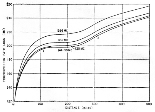
Fig. 1. Path loss vs. distance for amateur frequencies above 50 Mc. Values indicated are those that the path loss will be equal to, or less than, for 99 per cent of the hours of the year. This curve should be used for extreme reliability requirements.
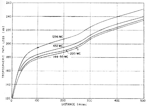
Fig. 2. Path loss vs. distance for 50 per cent of the hours of the year.
The first thing to be noted from the graphs is that the signal loss between two stations on the earth is anything but a straight line as the distance is increased. At first, the path loss increases rapidly as the distance becomes greater, then it ends to level out and again rise, but not as steeply as the original change of path loss. This is particularly true of the graph. for 99 per cent of the hours of the year. This means that for a given increase in power or antenna gain, the benefit which can be achieved depends on the distance to the station that is receiving you.
As an example, assume there is a low-power 2 meter station which can reliably work a similar station 60 mile away. Referring to Fig. 1 (99 per cent of the hours of the year), it can be seen that the path loss for 60 mile is about 180 dB. If the station transmitted power is raised from 6 watt to 60 watt, the station can now be heard reliably 90 mile away, since the 10 dB increase in power will overcome 10 dB of path loss, increasing allowable path loss from 180 to 190 dB. However, for an increase in power of 10 times, the distance worked is only increased by 1.5 times. Making another increase in power of 10 dB, thus raising the transmitted power from 60 to 600 watt, the allowable path loss is 200 dB and the working distance 240 miles. This time an increase in power of 10 times changed the station range 2.7 times, a substantial increase in distance from 90 to 240 mile.
This type of information can be very helpful if future station changes are planned. By the use of the method described here to determine where your station lies on the curve, the changes required to increase your working distance to a desired value can be easily found. Conversely, it is possible to determine if a planned change will accomplish the desired results.
It is a well-known fact that c.w. produces much better results than voice modulation in working v.h.f. DX. It becomes quite obvious why this is so by looking at Fig. 1. Take a typical 6-meter station: using a 100 watt transmitter and a 5 element beam, on phone, this station can probably work a similar station 110 mile away (see point 1, Fig. 1). The use of c.w. buys an additional 17 dB gain over the use of a.m. phone. Therefore, if this station switches to c.w. with no other changes he can now work another similar station at a distance of 310 mile (see point 2, Fig. 1). The switch to c.w. has pushed the station over the hump and produced a sizable increase in working distance.
If a comparison is made between Figs. 1 and 2, it is interesting to note that if you can tolerate being able to work a station only 50 per cent of the time instead of 99 per cent of the time, the maximum working distance is increased considerably. Using the previous example of the 6 meter 100 watt station, 99 per cent of the hours of the year he could work only 110 mile, but if the operator is satisfied with 50 per cent of the hours of the year he could work 250 mile (see point 3, Fig. 2).
Station gain
So much for looking at the effects. In order to estimate your station's capabilities, two basic calculations must be performed. The first is the determination of a number that will be called station gain; the second is the path loss. The station gain is made up of eight quantities receiver sensitivity, transmitted power, receiving antenna gain, receiving antenna height gain transmitting antenna gain, transmitting line loss, transmitting antenna height gain, am required signal-to-noise ratio. The value of station gain is obtained by determining the value of each of these quantities and converting them to a dB value, then adding the db. values tc obtain a total.
The computation of the station gain at first appears to be somewhat complicated, not due to the mathematics, but because of the various numbers which have to be obtained in order that their dB values may be added together. Two of the values are obtained by nomograms of Figs. 3 and 4. These are the receiver sensitivity and the antenna height gain. These and the other quantities are discussed one at a time with clues as to where the appropriate numbers may be found.
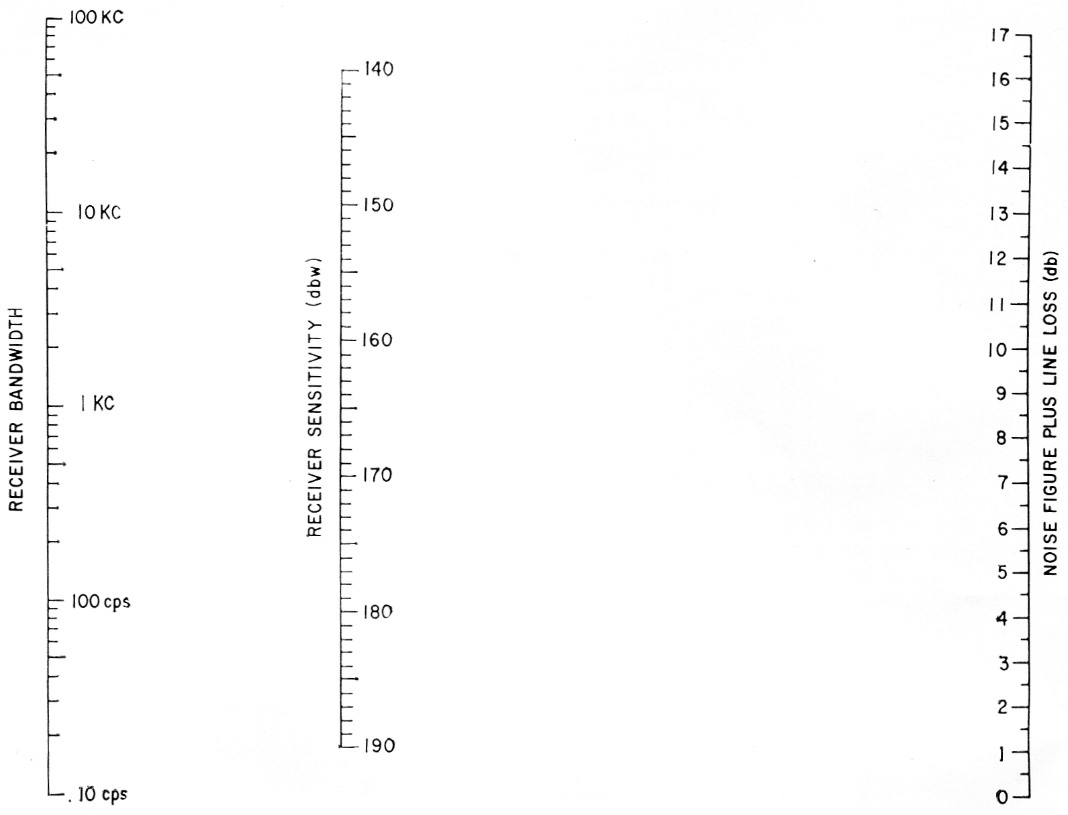
Fig. 3. Nomogram for finding effective receiver sensitivity.
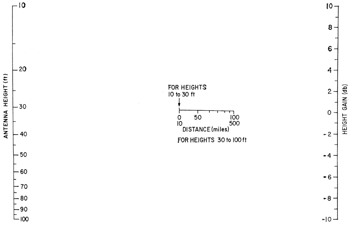
Fig. 4. Nomogram for determination of antenna-height gain.
Receiver sensitivity
The largest number in the station gain is the sensitivity of the receiver. The nomogram of Fig. 3 is used to calculate this. In order to determine the value, a straightedge is placed between the appropriate receiver bandwidth value on the left-hand scale and the noise figure of your converter, plus line-loss value, on the right-hand scale. The receiver sensitivity is then given on the center scale. The receiver bandwidth for phone will vary for the particular receiver, from approximately 2 to 10 kc. Your receiver instruction book probably will list the phone receiver bandwidth. This value should be used. If the receiver is used on c.w., due to the properties of the ear, the value of approximately 500 cycles proves best for the receiver bandwidth scale, regardless of the actual receiver bandwidth in the range from 3 kc to 100 cycles. Therefore, computations of phone signals use between 2 and 10 kc for the receiver bandwidth and 500 cycles for the receiver bandwidth for the reception of c.w.
The noise figure may be a little more difficult to determine. If you have a commercial converter, the instruction book may list its noise figure. If your converter is homemade, the noise figure could vary anywhere from 2 to 10 dB, depending on the tube type used in the front end and the frequency band. If you do not know the value of the noise figure of your receiver, one way to determine this is to look at the commercial converter specifications which have a tube line-up similar to yours. The back pages of QST are likely to have some of these converter ads. In addition to the noise figure, the line loss from the receiver to the antenna must be computed.
This is easily done by the use of the ARRL Handbook or Antenna Book, which list the transmission-line losses in dB per hundred foot, as a function of the frequency, for all common types of coaxial cable and open-wire line. By adding together the noise figure in db. and the line loss in dB, then drawing a line between this value and the chosen receiver bandwidth, the receiver sensitivity is obtained on the center scale. This number as noted on the chart is in dBw, meaning that it is a given number of dB below the reference level of 1 watt. To be strictly correct, a negative sign should be in front of these db. numbers, but it has been omitted since we are computing a value we will call station gain.
Antenna gain
The next largest number in the station gain is the gain of your transmitting antenna and the gain of the other station's receiving antenna, or vice versa. Of all the numbers used in the specifications of amateur radio equipment, the antenna gain is probably the one most loosely defined and the least likely to be believed. Therefore, for the antenna gain, although you can use the antenna gain as advertised by your antenna manufacturer (if you have a commercial antenna), probably a better and more conservative figure could be obtained by using a simple formula. The gain of a Yagi-type antenna is approximately equal to 10 times the boom length in wavelengths. This formula is independent of the number of elements.
Expressing this antenna gain in terms of length in foot and the frequency used:
![]()
where
Gp = Gain of the antenna expressed as a power ratio.
L = Length of the antenna in foot f = Frequency of station in megacycles
N = Number of stacked antennas of the same length stacked widely apart.
This number must then be converted into dB by the standard dB formula or by using the dB table in the Handbook. This is the gain of the antenna if it were in free space. However, since most antennas are operated over the ground and pointed at the horizon, an additional gain due to the earth's reflection should be added to this calculated antenna gain. This value should be around 4 dB for most u.h.f. antenna sites. Therefore, obtain the antenna gain by the formula or commercial specifications and add 4 dB to this number. If you have a collinear antenna you had better use the commercial specification, or a reasonable estimate, and then add the 4 dB for ground reflection.
Antenna-height gain
Because the nomogram for the calculation of path loss is based on an antenna height of 30 foot, receiving and transmitting, an additional nomogram is required in order to obtain the antenna-height gain if your antenna is of a height other than 30 foot. The antenna-height gain is a function of the distance to the station you are working and therefore the nomogram of Fig. 4 has a distance scale in the center. As noted on this scale, from 10 to 30 foot, all station distances are considered to be at the point indicated by the arrow; i.e., 10 mile. However, for antenna heights from 30 to 100 foot, the specific station distance should be used as a point through which to draw the line from your antenna height (left-hand scale) to obtain the height gain on the right-hand scale. It should be noted that the left-hand mark on the center distance scale is for distances from 0 to 10 mile and the right-hand mark of the distance scale holds for all distances from 100 to 500 mile.
To determine antenna-height gain, lay a straight-edge from the value of antenna height intersecting the station distance in the center of Fig. 4 and read the height gain on the right-hand scale.
Transmitter power
The transmitter power is an easy one to calculate. Since you know the power input you are running, convert this into the dB ratio referred to 1 watt, since the receiver sensitivity is referred to 1 watt. That is, your input power divided by 1 is used for your dB ratio calculation; or look it up in the dB table of the ARRL Handbook. Because the transmitter is not 100 per cent efficient, subtract 2 db. for efficiency in the 50 or 144 Mc bands and as much as 4 dB for the higher bands.
As an example, a 100 watt transmitter expressed in dB is equal to 20 dB, minus 2 dB for efficiency, or 18 dB.
Transmitter line loss
As with the receiving station line loss, this can be obtained by looking up the specific cable loss in the ARRL Handbook.
Required signal-to-noise ratio
Because all forms of modulation are not as efficient as c.w., a required signal-to-noise ratio must be subtracted from the station gain. For c.w., no additional signal-to-noise ratio is required, since this is used as a standard. For single sideband, subtract 3 dB from the station gain. For a.m., subtract 7 dB (The additional 10 dB, purely a bandwidth factor, is included in the nomogram, Fig. 3).
In addition to loss of signal due to the type of modulation, a fading loss must also be subtracted from the station gain. It has been shown that for station distances of over approximately 100 mile, a fade amplitude of 13.5 dB exists. This is a within-the-hour fade. The path loss curves are expressed as representing a given percentage of hours of the year, because withinthe-hour additional signal changes can be expected. The curves are for the average signal for any hour. Thus, since a 13.5 dB signal change will occur at some variable rate within a period of a few minutes, the signal will drop about 7 db. below the average and then rise 7 dB above the average. This fading is familiar to all v.h.f. operators. Although the rate of fade will be variable, the amplitude is constant. Therefore, in order to copy another station solidly it is necessary to subtract this 7 dB from the station gain. This holds for all distances greater than 100 mile. For distances shorter than 100 mile it drops off almost in a straight line. For a 50 mile station to station distance, subtract 3.5 dB, etc. Therefore, subtract from the station gain 0 dB for c.w. or 3 dB for s.s.b., or 7 dB for a.m., and an additional 7 dB for fading.
Having obtained the values required to obtain station gain as discussed above, the station gain is obtained from the following procedure:
- From Fig. 3 obtain receiving-station receiver sensitivity.
- Add transmitting-station power in dB.
- Add receiving-station antenna gain in dB.
- Add receiving-station antenna-height gain in dB (if it is negative, subtract it).
- Add transmitting-station antenna gain in dB.
- Add transmitting-station antenna-height gain in dB (watch that negative value).
- Subtract transmitting-station line loss in dB.
- Subtract required signal-to-noise ratio, 0 for c.w., or 3 dB for s.s.b., or 7 dB for a.m., and 7 dB for fading.
Path loss
The determination of path loss is considerably easier than the station gain. It is obtained by the use of the nomogram of Fig. 5. This is the same information as shown in Fig. 1, except that in nomogram form it is considerably more accurate. The use of this nomogram gives the path loss between two stations over a smooth earth for 99 per cent of the hours of the year. To determine the value of path loss, lay a straightedge from the value of distance between stations on the left-hand scale to the same distance on the appropriate right-hand distance scale and read off the value of path loss on the center scale. The right-hand distance scales are for the various amateur bands between 50 and 1300 Mc. However, note that some of the bands have incomplete right-hand distance scales. 1296 Mc has a complete distance scale. For 432 Mc, use the dot surrounded by the triangle as the distance scale. For 220 Mc, use the dot surrounded by the square. For 144 Mc, use the dot surrounded by the circle. For 50 Mc, use the dot surrounded by the circle for distances from 5 to 19 miles and from 90 to 500 miles. Use the scale as marked between 10 and 90 miles.
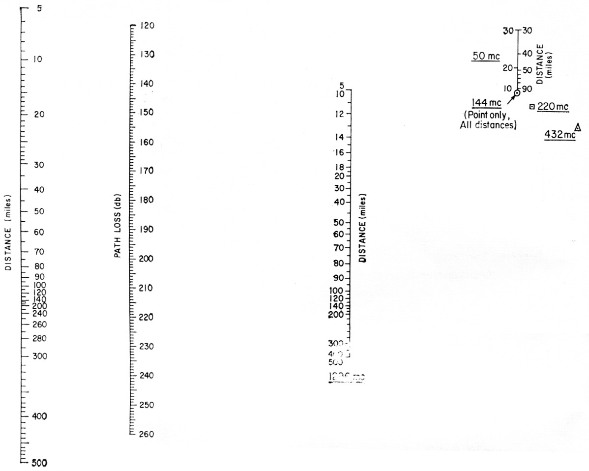
Fig. 5. Nomogram for finding distance capabilities of v.h.f. stations.
As an example, the path loss at a distance of 50 miles is 185 dB for 1296 Mc, 178 dB for 432 Mc, 176 dB for 220 Mc, 175 dB for 144 Mc, and 174 dB for 50 Mc.
This path-loss information can be used two ways. Choosing a distance between stations and then determining the path loss, this value subtracted from the station gain gives the signal strength at the receiver, over and above that required, expressed in dB. This can be converted to S units by dividing the dB value by 6. If the value is negative, the station is too far away to be worked.
If, in figuring the station gain as above, you use your own station receiver and transmitter parameters and use your antenna gain for both the receiving antenna gain and transmitter antenna gain, this will give the station gain for two similar stations. If this value of station gain is entered on the center scale of Fig. 5 as the path loss, and the straightedge adjusted to lie on same value on both left-hand and right-hand distance scales, and if a right-hand distance scale exists, this is the distance which can be worked by your station if a similar station to yours were at that distance. This calculation can be used to get an idea of how far you could expect to work other stations, unless some favorable propagation is present. It is also helpful for determining what result station changes produce.
One last consideration should be made when choosing the distance between stations. The nomogram of Fig. 5 is based on a smooth earth. If the terrain at the horizon at your location is higher or lower than your antenna, a correction can be made to the distance between stations in order that a more nearly correct path loss will be obtained. After determining the air-line distance between stations of interest, determine the horizon elevation angle in degrees in the direction of the station to be worked and multiply it by 69 mile. If the angle is positive, add this new value to the distance: if the angle is negative, subtract this distance from the actual disstance This correction should be made for both stations.
Examples
Determination of the signal strength above that required, from Station A to Station B:
| Station A Receiving | Station B Transmitting |
|---|---|
| Frequency: 144 Mc, c.w. Receiver noise figure: 3 dB Transmission line: 40 ft RG-8 Receiver bandwidth: 500 cycles Antenna: 14 ft boom Antenna height: 20 ft Horizon angle: +1.2° |
Distance: 200 mile Transmitter power: 250 watt Transmitter line: 100 ft RG-8 Antenna: 2 Yagis 28 ft long Antenna height: 65 ft Horizon angle: -0.5° |
Preliminary calculations
a) Looking up transmission-line loss in the ARRL Handbook, you find 1.0 dB for the receiver and 2.5 dB for the transmitter.
b) Compute antenna gain G = 20.6, or 13 dB for the receiver. G = 82 or 98 19 dB for the transmitter.

Then find station gain:
1) Receiver sensitivity (Fig. 3), 500 cycle and 4 dB:    172.5 dB
2) Transmitter power, 24 - 2 dB:                          22   dB
3) Receiver antenna gain, 13 dB + 4 dB:                   17   dB (4 dB for earth reflection)
4) Receiver antenna-height gain (Fig. 4):                 -3.2 dB
5) Transmitter antenna gain, 19 dB + 4 dB:                23   dB
6) Transmitter antenna-height gain (Fig. 4):              +3.2 dB
7) Transmitter line loss:                                 -2.5 dB
8) Required signal-to-noise ratio, c.w.:                   0   dB
9) Fading:                                                -7   dB
                                                         ----------
Total Station Gain =                                     225   dB
Path Loss Computation
Find distance correction:
a) Multiply 1.2° × 69 =     82.8 mile
   Multiply -0.5° × 69 =   -31.5
                          ------------
Total correction =          48.3 mile

b) Find effective distance:
200 + 48 = 218 mile

Find path loss:
1) Lay straightedge from 248 miles on left-hand distance scale to the dot surrounded by a circle (114 Mc.) on the right-hand scale.
Find path loss = 203.5 dB

Find signal strength above that required:
1) Station gain =         225  dB
   Path loss =          -203.5 dB
Signal above required =   21.5 dB or in S units, 21.5 / 6 = 3.6 S units.
Determination of maximum range of two stations of similar equipment
Frequency: 1296 Mc., a.m. phone
Receiver noise figure: 9 dB
Transmission line: 60 ft RG-11.
Receiver bandwidth: 3 kc
Antenna: 4 ft. boom, Yagi
Antenna height: 40 ft
Transmitter power: 50 watt
Horizon angle: 0 degrees
Distance = ?
Preliminary calculation
a) Looking up transmission line in ARRL Handbook, you find 60 ft RG-11 =    4.8 dB
b) Compute antenna gain:                                                   17.2 dB

Find station gain:
1) Receiver sensitivity (Fig. 3), 3 kc. and 13.8 dB:                      155   dB
2) Transmitter power, 17 dB - 4 dB:                                       -13   dB (-4 dB because of low efficiency at 1296)
3) Receiver antenna gain, 17 dB + 4 dB:                                    21   dB
t) Receiver antenna height gain (Fig. 4):             (distance unknown but 1.5 dB guess 80 mile)
5) Transmitter antenna gain, 17 dB + 4dB:                                  21   dB
6) Transmitter antenna height gain:                                         1.5 dB
7) Transmitter line loss:                                                  -4.8 dB
8) Required signal-to-noise ratio: a.m.                                    -7   dB
   fading                                                                  -7   dB
                                                                          ----------
Total station gain=                                                       194.2 dB
A method
Distance determination
Using Fig. 5, enter center scale (path loss) with 194 dB and adjust straightedge for equal distance on left-hand distance scale and 1296 Mc distance scale. Find station working distance = 66 mile. If the distance was guessed wrong on the height gain nomogram, the new distance just obtained should be used in the height gain nomograph and a new answer obtained to correct the station gain.
Future use
Once you have determined t he valises for your own station, mark them down and then you won't have to look them up again. This will make future computations easier.
Next time you plan to make a station change, make a computation of your "similar station" working distance, and see if it produces the desired result. Maybe just a small change can get you "over the hump" of Fig. 1.
Notes
- Norton, "System loss in radio wave propagation," Journal of Research of the National Bureau of Standards, July-August, 1959.
D.W. Bray, K2LMG.