Smith-chart calculations for the radio amateur 2
Determining actual antenna impedances
To determine an actual antenna impedance from the Smith Chart, the procedure is similar. The electrical length of the feed line must be known, and the impedance value at the input end of the line must be determined through measurement. In this case, the antenna is connected to the far end of the line and becomes the load for the line. Whether the antenna is intended purely for transmission of energy, or purely for reception makes no difference; the antenna is still the terminating or load impedance on the line as far as these measurements are concerned. The input or generator end of the line would be that end connected to the device for measurement of the impedance. In this type of problem, the measured impedance is plotted on the Chart, and the TOWARD-LOAD wavelengths scale is used in conjunction with the electrical line length to determine the actual antenna impedance.
For example, assume we have a measured input impedance to a 50-ohm line of 70 - j25 ohms. The line is 2.35 wavelengths long, and is terminated in an antenna. We desire to determine the actual antenna impedance. Normalize the input impedance with respect to 50 ohms, which comes out 1.4 - j0.5, and plot this value on the Chart. See Fig. 7. Draw a constant-s.w.r. circle through the point, and transfer the radius to the external scales. The s.w.r. of 1.7 may be read from the S.W.V.R. scale (at A). Now draw a radial line from prime center through this plotted point to the wavelengths scale, and read a reference value, which is 0.195 (at B), on the TOWARD-LOAD scale. Remember, we are starting at the generator end of the transmission line.
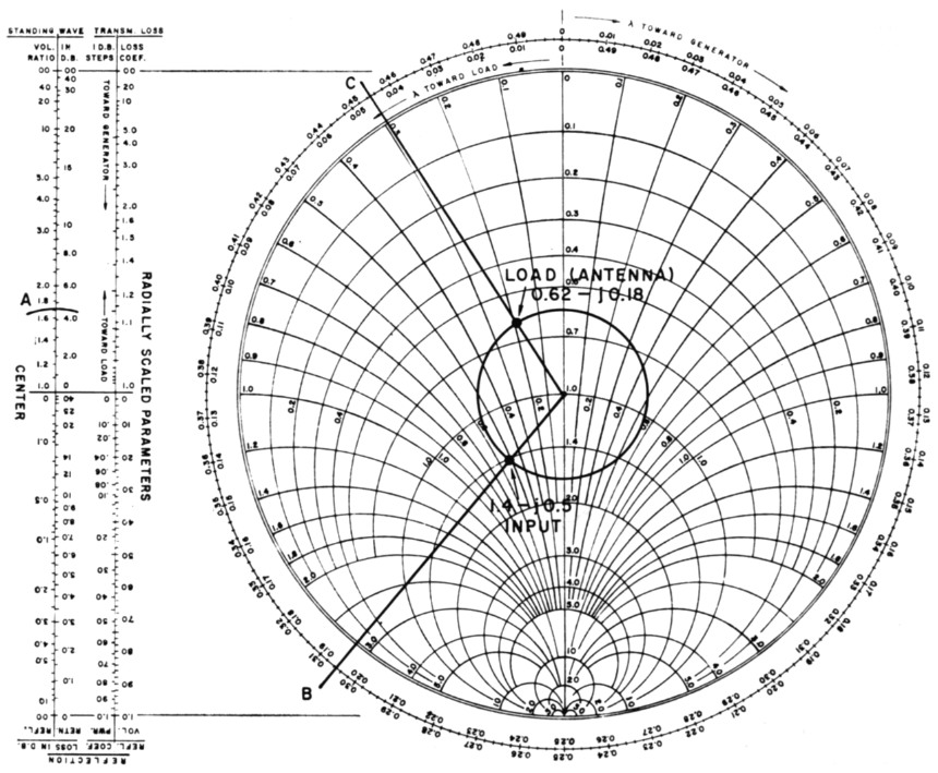
Fig. 7.
To locate the load impedance on the s.w.r. circle, we add the line length, 2.35 wavelengths, to the reference value from the wavelengths scale, and locate the new value on the TOWARDLOAD scale; 2.35 + 0.195 = 2.545. However, the calibrations extend only from 0 to 0.5, so we must subtract a whole number of half wavelengths from this value and use only the remaining value. In this situation, the largest integral number of half wavelengths that can be subtracted is 5, or 2.5 wavelengths. Thus, 2.545 2.5 = 0.045, and the 0.045 value is located on the TOWARD-LOAD scale (at C). A radial line is then drawn from this value to prime center, and the coordinates at the intersection of the second radial line and the s.w.r. circle represent the load impedance. To read this value closely, some interpolation between the printed coordinate lines must be made, and the value of 0.62 - j0.18 is read. Multiplying by 50, the actual load or antenna impedance is 31 - j9 ohms, or 31 ohms resistance with 9 ohms capacitive reactance.
Problems may be entered on the chart in yet another manner. Suppose we have a length of 50-ohm line feeding a resonant quarter-wave vertical ground-plane antenna. Further, suppose we have an s.w.r. monitor in the line, and that it indicates an s.w.r. of 1.7 to 1. The line is known to be 0.95 wavelength long. We desire to know both the input and the antenna impedances.
From the data given, we have no impedances to enter onto the chart. We may, however, draw a circle representing the 1.7 s.w.r. See Fig. 8. We also know, from the definition of resonance, that the antenna presents a purely-resistive load to the line; i.e., no reactive component. Thus, the antenna impedance must lie on the resistance axis. By observing the Chart with only the s.w.r. circle drawn, we see two points which satisfy this requirement in Fig. 8. These points are 0.59 + j0 and 1.7 + j0. Multiplying by 50, these values represent 29.5 and 85 ohms resistance. This may sound familiar, because the ARRL Handbook tells us that when a line is terminated in a pure resistance, the s.w.r. in the line equals ZR/Zo or Zo/ZR, where ZR = load resistance and Zo = line impedance.
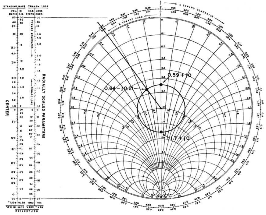
Fig. 8.
If we consider antenna fundamentals, we know that the theoretical impedance of the ground-plane antenna is approximately 36 ohms. We therefore can quite logically discard the 85-ohm impedance figure in favor of the 29.5-ohm value. This is then taken as the actual load-impedance value for the Smith Chart calculations. The line input impedance is found to be 0.64 - j0.21, or 32 - j10.5 ohms, after subtracting 0.5 wavelength from 0.95, and finding 0.45 wavelength On the TOWARD-GENERATOR scale. (The wavelength reference in this case is 0.)
Determination of line length
In the example problems given so far, the line length has conveniently been stated in wavelengths. The electrical length of a piece of line depends upon its physical length, the radio frequency under consideration, and the velocity of propagation in the line. If an impedance-measurement bridge is capable of quite reliable readings at high line-s.w.r. values, the line length may be determined through line input-impedance measurements with short- or open-circuit terminations. A more direct method is to measure the line's physical length and apply the value to a formula. The formula is:
![]()
where:
N = Number of electrical wavelengths in the line,
L = Line length in feet,
F = Frequency in megacycles, and
K = Velocity or propagation factor of the line.
The factor K may be obtained from transmissionline-data tables, such as appear in the Handbook in the chapter on transmission lines. Common coaxial cables with solid dielectric, such as RG-8, 9, 11, 17, 19, 58, 59 and 83 have a velocity or K factor of 66.9 per cent. Teflon-dielectric, or combination solid- and air-dielectric lines, have a higher velocity factor - up to 93 per cent for some special types of coaxial line. Most 300-ohm receiving-type balanced Twin-Lead has a velocity factor of 82 per cent; 75-ohm receiving-type ribbon line 68 per cent, transmitting type 71 per cent. Open-wire lines and ladder-type TV lines will exhibit a velocity factor of 97 to 97.5 per cent. All types of line having a solid dielectric can vary in velocity factor from the values given here, depending on the age and condition of the dielectric material. As the dielectric deteriorates, the velocity factor will become lower, and usually the associated dielectric losses will become higher. This is especially true of ribbon-type lines, where the dielectric material is exposed directly to the weather in most installations. In applying the velocity factor to the formula, the percentages must be converted to their decimal equivalent.
Line-loss considerations
The problems presented so far have ignored attenuation, or line losses. Quite frequently it is not even necessary to consider losses when making calculations; any difference in readings obtained would be almost imperceptible on the Smith Chart. When the line losses become appreciable, as with very long lines in terms of wavelengths, or with high s.w.r. values, loss considerations may be warranted. This involves only one simple step, in addition to the procedures previously presented.
Because of line losses, the s.w.r. does not remain constant throughout the length of the line. Power reflected from a mismatched load is attenuated as the wave travels toward the generator. As a result, there is a decrease in s.w.r. as one progresses away from the load. To truly represent this situation on the Smith Chart, instead of drawing a constant s.w.r. circle, it would be necessary to draw a spiral inward and clockwise from the load impedance toward the generator. The rate at which the curve spirals toward prime center is related to the attenuation in the line. Rather than drawing spiral curves, a simpler method is used in solving line-loss problems, by means of the external scale TRANSMISSION-LOSS, 1-DB. STEPS in Fig. 9. Because this is only a relative scale, the db. steps are not numbered.
If we start at the top end of this external scale and proceed in the direction indicated toward generator, the first db. step is seen to occur at a radius from center corresponding to an s.w.r. of about 9 (at A); the second db. step falls at an s.w.r. of about 4.5 (at B), the third at 3.0 (at C), and so forth, until the 15th db. step falls at an s.w.r. of about 1.05 to 1. This means that a line terminated in a short or open circuit (infinite s.w.r.) and having an attenuation of 15 db., would exhibit an s.w.r. of only 1.05 at its input. It will be noted that the db. steps near the lower end of the scale are very close together, and a line attenuation of 1 or 2 db. in this area will have only slight effect on the s.w.r. But near the upper end of the scale, 1- or 2-db. loss has considerable effect on the s.w.r.
In solving a problem utilizing line-loss information, it is necessary only to modify the radius of the s.w.r. circle by an amount indicated on the TRANSMISSION-LOSS, 1 dB STEPS scale. This is accomplished by drawing a second s.w.r. circle, of either greater or lesser radius than the first, as the case may be.
Assume that we have a 50-ohm line 0.282 wavelength long, with 1 dB inherent attenuation.
The line input impedance is measured as 60+j35 ohms. We desire to know the s.w.r. at the input and at the load, and the load impedance. As before, we normalize the 60 + j35-ohm impedance, plot it on the Chart, and draw a constant-s.w.r. circle and a radial line through the point. In this case, the normalized impedance is 1.2 + j0.7. From Fig. 9, the s.w.r. at the line input is seen to be 1.9 (at D), and the radial line is seen to cross the TOWARD-LOAD scale at 0.328 (at E). To the 0.328 we add the line length, 0.282, and arrive at a value of 0.610. To locate this point on the TOWARD-LOAD scale, first subtract 0.500, and locate 0.110 (at F); then draw a radial line from this point to prime center.
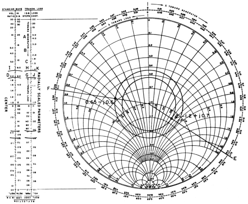
Fig. 9.
To account for line losses, transfer the radius of the s.w.r. circle to the external 1-05.-STEPS scale. This radius will cross the external scale at G, the fifth db. mark from the top. Since the line loss was given as 1 db., we strike a new radius (at H), one "tick mark" higher (toward load) on the same scale. (This will be the fourth db. tick mark from the top of the scale.) Now transfer this new radius back to the main chart, and scribe a new s.w.r. circle of this radius. This new radius represents the s.w.r. at the load, and is read as about 2.3 on the external S.W.V.R. scale. At the intersection of the new circle and the load radial line, we read 0.65 - j0.6 as the normalized load impedance. Multiplying by 50, the actual load impedance is 32.5 - j30 ohms. The s.w.r. in this problem was seen to increase from 1.9 at the line input to 2.3 (at I) at the load, with the 1-db. line loss taken into consideration.
In the example above, values were chosen to fall conveniently on or very near the "tick marks" on the 1-DB. scale. Actually, it is a simple matter to interpolate between these marks when making a radius correction. When this is necessary, the relative distance between marks for each db. step should be maintained while counting off the proper number of steps.
The total losses in a given piece of transmission line are dependent upon several factors, primarily frequency, line length, and s.w.r. Transmission-line data tables show " matched-line " losses for various types of lines at various frequencies, usually expressed in decibels per hundred feet. RG-8/U, for example, has an attenuation of 0.28 db. per hundred feet at 3.5 Mc., 0.65 db. at 14 Mc., 0.98 db. at 28 Mc., 2.65 db. at 150 Mc., and so on. The A.R.R.L. Antenna Book has quite complete tables of common transmission-line data. Attenuation for a given piece of line may be computed from table data; the attenuation in db. is directly proportional to the line length.
Adjacent to the 1 dB STEPS scale lies a Loss-COEFFICIENT scale. This scale provides a factor by which the matched-line loss in db. should be multiplied to account for the increased losses in the line when standing waves are present. These added losses do not affect the standing-wave ratio or impedance calculations; they are merely the additional dielectric and copper losses of the line caused by the fact that the line conducts more average current and must withstand more average voltage in the presence of standing waves. In the above example and in Fig. 9, the loss coefficient at the input end is seen to be 1.21 (at J), and 1.39 (at K) at the load. As a good approximation, the loss coefficient may be averaged over the length of line under consideration; in this case, the average is 1.3. This means that the total losses in the line are 1.3 times the matched loss of the line (1 dB), or 1.3 dB
Two additional external scales may find limited use in amateur applications. These are the REFLECTION-LOSS IN DB. scales. Both of these scales are related to the REFLECTION COEFFICIENT OF POWER scale, but express values in db., rather than in a power ratio. The RETURN scale expresses the ratio of total forward power to reflected power in db. This is sometimes called the reflection loss, although it does not necessarily represent an actual loss of power. If an impedance match is made at the sending end of the transmission line with a generator or a transmitter, a "reflection gain" takes place which neutralizes the "loss" at the load end. The REFLECTED scale expresses the ratio of total forward power to nonreflected power in db. This would represent the power consumed in the load (or power radiated by an antenna, plus ohmic losses), referenced to the total forward power in the line.
Summary
To summarize briefly, any calculations made on the Smith Chart are performed in four basic steps, although not necessarily in the order listed.
- Normalizing and plotting a line input (or load) impedance, and constructing a constant s.w.r. circle.
- Applying the line length to the wavelengths scales.
- Determining attenuation or loss, if required, by means of a second s.w.r. circle.
- Reading normalized load (or input) impedance, and converting to impedance in ohms.
The Smith Chart may be used for many types of problems other than those presented as examples. The transformer action of a length of line - to transform a high impedance (with perhaps high reactance) to a purely resistive impedance of low value - was not mentioned. This is known as "tuning the line," for which the Chart is very helpful, eliminating the need for cut-and-try procedures. The Chart may also be used to calculate lengths for shorted or open matching stubs in a system. In fact, in any application where a transmission line is not perfectly matched, the Smith Chart can be of value.
The Chart can also be used in solving other types of problems which were not brought into the scope of this article. Such problems include the use of the Chart for admittance, conductance, and susceptance calculations, or the computation of equivalent series or parallel components of an impedance or admittance. In short, the Smith Transmission Line Calculator or Chart is a very versatile tool for either amateur or professional use.
Part 1 - Part 2
Gerald L. Hall, K1PLP, EX-KH6EGL.