Match bandwidth of resonant antenna systems
Did you know that deliberately mismatching an antenna to its feed line can increase its SWR bandwidth? Here's how it works.
Half-wave dipoles, quarter-wave verticals and full-wave loops are all resonant antennas, as are some off-center-fed (OCF) antennas.(1) In most applications, we want to use these antennas over a frequency band near the antenna's resonance. In this article, match bandwidth is defined as the frequency band over which the SWR measured at the transmitter is less than 2:1. (Match bandwidth as defined here is often referred to as "2:1 SWR bandwidth.") In the remainer of this article, the word bandwidth means "match bandwidth."
Many hams think that maximum bandwidth is achieved with resonant antennas when a perfect match occurs near the center of the band of interest. This is not so. As I'll show, some mismatch at the center of the band provides wider bandwidth (although the increase is usually small). Further, the optimum amount of mismatch, and the achievable bandwidth, depend on feed-system losses. Perhaps most significantly, the bandwidth increase caused by feed-system loss can be very large.
You can gain more insight by thinking of the antenna and the transmission line as an antenna system. The bandwidth we're interested in is that measured at the transmitter end of the feed line. This is important because it's a measure of the band of frequencies over which your transmitter or amplifier can generally be used without an antenna tuner. We'll focus on bandwidth at the transmitter, and the match required at the antenna to achieve that bandwidth. It's important to keep this distinction in mind.
The antenna-system model
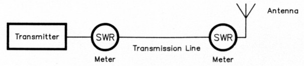
Fig 1 - The antenna system consists of a lossy transmission line and a simple resonant antenna load. The SWR meters are shown to emphasize that the SWR at the transmitter end and antenna end of the transmission line differ, as discussed in this article.
To explain this, I'll use the simple antenna system shown in Fig. 1. It consists of a transmission line and a resonant antenna. (The analysis is valid if a transformer, such as a 4:1 balun, is included in the model.) Fig 2 shows the antenna's equivalent circuit near resonance. Although the series RLC circuit is an approximation, it is close enough to the actual antenna impedance for the purpose of this discussion.
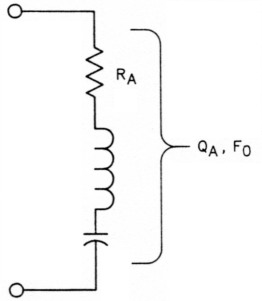
Fig 2 - The equivalent circuit of a resonant antenna. The simple series R-L-C approximation applies to many resonant antenna types, such as dipoles, monopoles, loops and antennas based on them. RA, QA and F0 are properties of the entire antenna, as discussed in the text.
For this analysis, the antenna can be described using only three parameters: resonant frequency (F0), antenna resistance (RA), and antenna Q (QA). RA is the antenna impedance at resonance and QA describes the energy-storage properties of the antenna.(2) Antenna Q is a useful concept because it is inversely proportional to antenna bandwidth; ie, the higher the QA, the lower the bandwidth, and vice versa. You can determine these quantities from simple SWR measurements.(3)
Near resonance, the SWR of a resonant antenna has the familiar bowl shape of Fig 3. There are two cases to consider:
- If Z0 is greater than RA, then SWRANTMIN = Z0 ÷ RA
- If Z0 is less than RA, then SWRANTMIN = RA ÷ Z0
where Z0 is the characteristic impedance of the transmission line and SWRANTMIN is the antenna's SWR at its resonant frequency, F0. (Throughout the remainder of this article, SWRANT means SWRANTMIN unless specified otherwise.)
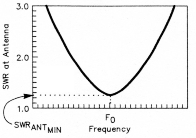
Fig 3 - SWR at the antenna versus frequency in the vicinity of resonance.
It's important to recognize that these two cases exist. I'll show that, for a given mismatch at resonance (SWRANT), Case 1, in which the feed-line impedance is higher than that of the antenna, always yields wider bandwidth than Case 2, where the antenna impedance is higher than that of the feed line.
Optimizing match bandwidth - in a nutshell
In sum, this article concludes that:
- Maximum bandwidth is not achieved when an antenna is matched to its transmission line at resonance.
- For a given mismatch at the antenna, wider bandwidth is always obtained (for the kinds of resonant antennas treated here) when the characteristic impedance of the line is higher than the antenna's impedance at resonance.
- Bandwidth is relatively insensitive to match at the antenna when the transmission line's characteristic impedance is higher than the antenna's impedance at resonance.
- The amount of mismatch at the antenna required to obtain maximum bandwidth depends on line loss.
- When the transmission-line loss is small, mismatching the antenna to obtain maximum bandwidth is not worthwhile; the bandwidth improvement over that attainable with a perfect match is small.
- Bandwidth is highly dependent on line loss, and very wide bandwidths may be obtained when the line loss is high.
- When line loss is high, deliberately mismatching the antenna can be advantageous, not only to increase match bandwidth, but also to reduce transmission-line loss over most of the band. This is especially true at VHF and UHF.
- Using a lossy transmission line to increase antenna-system bandwidth is not advisable, because lossy lines attenuate desired signals and worsen system noise figure (these are especially important to avoid at and above VHF).
- Unintentionally high transmission-line loss causes wide bandwidths in some antenna systems. - AI1H
Normalized frequency offset and normalized bandwidth
Frequency normalization is simply a process of multiplying all frequency-specific information by a constant to make the results more general. If we define the normalized frequency offset, ΔfN, as (QA ÷ F0) times the frequency departure from resonance, the results are very general. In other terms.
ΔfN = (QA ÷ F0) (f - F0) (Eq 1)
where f is the operating frequency.
This frequency-offset normalization lets us apply the general results described here to any resonant antenna, because QA and F0 are properties of the antenna itself. This normalization is valid when the frequency offset is small compared to the antenna's resonant frequency, which is usually the case.
We can use a similar normalization for bandwidth. Normalized bandwidth, BN, is defined as:
BN = (QA ÷ F0) BW (Eq 2)
where BW is antenna bandwidth.
For a particular antenna, QA and F0 are fixed, so BN is proportional to bandwidth, BW. Normalized bandwidth is useful because it applies to any resonant antenna.
SWR as a function of frequency
For the simple antenna system considered here, the only adjustable parameters are the antenna's resonant frequency and the match at the antenna at resonance. The desired resonant frequency is usually reached by adjusting antenna length, tuning a loading coil, or similar adjustments. The match at resonance can be adjusted in several familiar ways, depending on the specific antenna architecture:
- Setting of a T or gamma match.
- An impedance transformer or an LC matching network at the antenna.
- A transmission-line matching network, such as a Q-match or matching stubs.
- Selection of the feed-point position of an off-center-fed antenna.(4)
- Positioning of a tap on a coaxial-resonator match.(5)(6)
Fig 4A shows the SWR at the transmitter versus normalized frequency offset for very short or lossless transmission lines. A mismatch at the antenna provides maximum bandwidth at the transmitter end of the feed line. Three cases are shown:
- The optimum-mismatch condition (achieved when Z0 is higher than RA).
- The case when a perfect match exists at resonance.
- The same SWR at resonance as the optimum-mismatch condition, except that Z0 is less than RA.
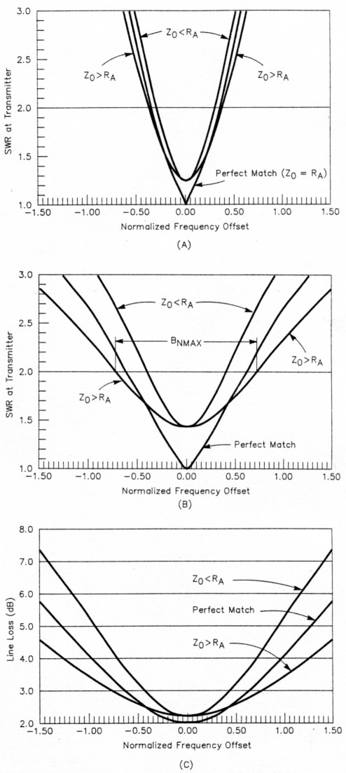
Fig 4 - SWR at the transmitter and transmission-line loss versus normalized frequency offset: (A) SWR for the lossless transmission line case; (B) SWR when the matched line loss is 2 dB; and (C) actual line loss when the matched line loss is 2 dB. The equations on which the figures are based are provided in the Appendix.
Figs 4B and 4C show the pronounced effect of a lossy transmission line. Specifically, the line has a matched loss of 2 dB (matched loss is the loss in a transmission line that's terminated in its characteristic impedance, Z0). Matched loss is a useful parameter because its value can be calculated from published data and line length. Fig 4B shows SWR at the transmitter, and Fig 4C shows actual line loss. A line with 2 dB loss is used as an example because it helps to clarify some of the points I want to make. The graphs that follow show the results for other matched-loss values.
It's worthwhile to study Fig 4, where the same normalized-frequency-offset scale is used in all three graphs. When the matched line loss is small, the differences for the three cases are small (Fig 4A). The large increase in bandwidth attributable to line loss is clearly illustrated. (Compare Figs 4A and 4B). Case 1, in which Zo is higher than RA, has a bandwidth advantage over Case 2. Fig 4C reveals an important reason for designing an antenna so that Case 1 matching occurs at the antenna: doing so keeps transmission-line loss to a minimum. Low line loss is important in certain applications, especially at VHF and UHF, where the antenna-system losses have a dramatic impact on system performance.
Bandwidth at the transmitter versus SWR at the antenna at resonance
As shown in Fig 3, SWRANT is a measure of the mismatch between the antenna and the transmission line at resonance. When the antenna is perfectly matched at resonance (Z0 = RA), the SWR is 1:1 at both ends of the line, regardless of the line loss. Except in this special case, whenever line loss exists, the SWR at the transmitter will be less than the SWR at the antenna. Therefore, it follows that an antenna fed with a lossy transmission line will have a wider match bandwidth at the transmitter than at the antenna, because the transmitter-end SWR at the antenna's 2:1 points will always be less than 2:1.(7)
Fig 5 shows normalized bandwidth at the transmitter as a function of antenna mismatch at resonance. First, look at the lossless-line case. The bandwidth is maximum when SWRANT (and SWRTX, the SWR at resonance at the transmitter end of the cable) = 1.25, not when a perfect match exists at resonance. Note also that the optimum mismatch occurs when Z0 is higher than RA.(8)(9) This result is predictable because the antenna impedance rises on either side of resonance. By starting with an impedance at resonance that's higher than Z0, the feed-point match gets worse faster than if the impedance at resonance was less than Z0. For a given value of SWRANT, the Case 1 bandwidth is always SWRANT times the Case 2 bandwidth.
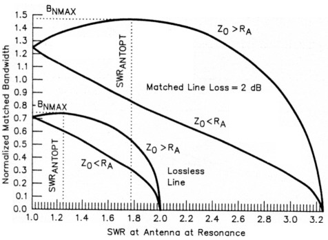
Fig 5 - Normalized bandwidth versus mismatch at the antenna at resonance. Note that the bandwidth is always greater when the feed line's characteristic impedance (Z0) is higher than the antenna's resonant resistance (RA).
Here's an example of how you can use the results shown in Fig 5. Suppose the antenna is an 80-meter dipole resonant at 3.8 MHz and with a Q of 13 (F0 = 3.8 MHz and QA = 13). The maximum bandwidth is obtained by using the fact that the actual bandwidth is (F0 - QA) times the normalized bandwidth. If the line is loss-less, the maximum normalized bandwidth is 0.75. Therefore, the antenna's actual maximum bandwidth is (F0 - QA) x 0.75, or (3800 kHz ÷ 13) x 0.75, or 219 kHz.
When the line has loss, the situation is similar. Also in Fig 5, normalized bandwidth is plotted as a function of SWRANT for the case when the matched line loss is 2 dB. For the same example (F0 = 3.8 MHz and QA = 13), the maximum normalized bandwidth is 1.466, so the actual maximum bandwidth is (3800 kHz ÷ 13) x 1.466, or 428 kHz - almost twice the bandwidth of the lossless-line case.
Fig 5 shows several interesting things. First, it graphically illustrates the bandwidth advantage of Case 1 (where Z0 is higher than RA) over Case 2 (in which Z0 is less than RA). Also, the SWRANT value that yields maximum bandwidth increases as line loss increases. The most striking message, however, is how much the maximum bandwidth increases as line loss increases. This is what causes such wide bandwidths in some antenna systems. In fact, some manufacturers use lossy matching networks and resistive attenuators in their antennas for the specific purpose of increasing bandwidth. Particularly in some commercial applications, trading loss for bandwidth is an acceptable - or even necessary - compromise. Be aware, however, of the signal loss that results from such a compromise.
Note that Fig 5's bandwidth-versusmismatch curves for Case 1 (Z0 > RA) are broadly peaked. In fact, the curves are symmetrical around SWRANT = SWRANTOPT. For the lossless-line case, the bandwidth is the same at SWRANT = 1.5 as it is at SWRANT = 1. For the case in which the matched line loss is 2 dB, the bandwidth is the same at SWRANT = 2.55 and SWRANT = 1.
Optimum mismatch
The values of SWRTX and SWRANT that provide the maximum bandwidth, SWRTXOPT and SWRANTOPT, respectively, are shown as a function of line loss in Fig 6. This result is independent of antenna Q. This graph is useful when you're designing resonant antenna systems for maximum bandwidth.(10)
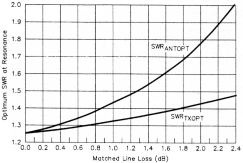
Fig 6 - Optimum mismatch at the antenna at resonance (SWRANTOPT) and the resultant SWR at the transmitter (SWRTXOPT) to achieve maximum antenna-system bandwidth at the transmitter.
Comparison: perfect match at resonance versus maximum bandwidth
Although maximum bandwidth is achieved when there is a deliberate mismatch at the antenna at resonance, it is important to put things in perspective. Just how much bandwidth is sacrificed when the antenna is perfectly matched to the feed line at resonance (Z0 = RA)? The answer to this question depends on the feed-line loss, as shown in Fig 7, where the bandwidth increase possible over that when a perfect match exists at resonance is plotted as a function of matched line loss. For very low line loss, the advantage is only a 6% bandwidth gain. In this situation, the deliberate mismatch is hardly worth the effort.
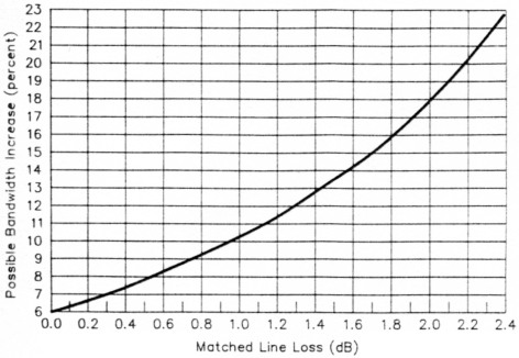
Fig 7 - Bandwidth increase possible by deliberately mismatching an antenna at resonance.
The advantage increases, however, when the line loss increases. For example, if the matched line loss is 2 dB, the bandwidth increase that results from deliberately mismatching the antenna is a substantial 18%. Fig 4B illustrates this improvement.
When you're designing an antenna system, it's important to weigh the relative importance of increasing bandwidth against achieving a better match over a smaller band. In many cases, the maximum achievable bandwidth is not required, and it may be more important to have a lower line loss. This occurs when the SWR at the antenna is close to 1:1. Hence, when the operating band is much smaller than the maximum possible bandwidth, it is more desirable to aim for a perfect match at resonance than to increase the system bandwidth at the cost of higher SWR at resonance.
Bandwidth at the transmitter and transmission-line loss
Fig 8 shows normalized bandwidth for a given matched line loss. Two important cases are shown: when perfect match exists at resonance (SWRANT = 1:1); and the maximum-bandwidth case. The advantage of the maximum-bandwidth case over the perfect-match case increases as matched line loss increases, as discussed earlier.
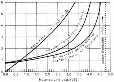
Fig 8 - Normalized bandwidth and band-edge line loss versus matched line loss.
Note that the bandwidth is infinite when the matched loss is greater than 4.77 dB. This is because the reflected wave is attenuated enough by the line loss so that the SWR is always less that 2:1.(11) This result is independent of antenna impedance.
As shown in Fig 8, very large bandwidths are attainable with larger line losses. The penalty, of course, is line loss, which is also shown in Fig 8. Here the actual line loss (not the matched loss) at the band edges (where SWR = 2:1) is plotted. Note from the curve that the band-edge line loss is just under 3 dB when the matched line loss is 2 dB.
These graphs bring home the fact that we should be aware of the losses in our antenna systems. In some applications, it may be more desirable to sacrifice some bandwidth to achieve a closer match (and hence lower loss) over a smaller portion of the band.
Summary
By analyzing a resonant antenna and its transmission line as an antenna system, some useful conclusions regarding bandwidth emerge. Although deliberate mismatch at the antenna can yield more bandwidth at the transmitter, the gain over a perfect match at resonance is usually small. However, line loss can have a large effect on bandwidth.
I do not advocate using a lossy transmission line to achieve wide bandwidth. High line loss certainly explains the wide bandwidths of some antenna installations, however.
When designing an antenna system, don't fall into the "low SWR at all costs" trap. SWR is not necessarily an indication of system performance. The material included here is complementary to that provided by Walt Maxwell, W2DU.(12) His book, Reflections, is recommended reading for all antenna buffs, because it establishes the correct perspective for antenna matching.
Appendix
The following equations were used to plot the graphs shown in this article. They may be useful for analyzing other antenna systems.
• Matched transmission line power loss ratio, k:
![]()
where A0 = matched line loss in dB
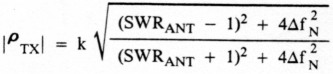
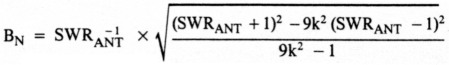
• SWR at the transmitter versus normalized frequency offset (Figs 4A and 4B):
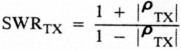
where ρTX = reflection coefficient at the transmitter.
Case 1 (Z0 > RA):
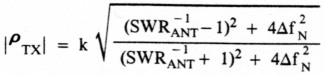
Case 2 (Z0 < RA):
• Transmission-line loss versus normalized frequency offset (Fig 4C):
![]()
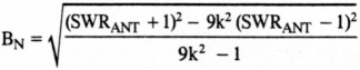
• Normalized bandwidth versus mismatch at resonance (Fig 5):
Case 1 (Z0 > RA):
Case 2 (Z0 < RA):
• Optimum mismatch versus matched line loss (Fig 6):
At the antenna: 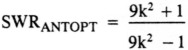
At the transmitter: ![]()
• Bandwidth increase versus matched line loss (Fig 7):
Percent Bandwidth Increase = 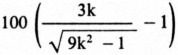
• Maximum normalized bandwidth versus matched line loss (Fig 8):
![]()
• Normalized bandwidth when a perfect match exists at resonance versus matched line loss (Fig 8):
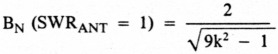
• Band-edge line loss versus matched line loss (Fig 8):
![]()
Notes
- F. Witt, "How to Design Off-Center-Fed Resonant Wire Antennas Using That Invisible Transformer in the Sky," in preparation for The ARRL Antenna Compendium, Volume 3.
- F. Witt, "Optimum Lossy Broadband Matching Networks for Resonant Antennas," RF Design, Apr 1990, p 44.
- F. Witt, "The Coaxial Resonator Match," The ARRL Antenna Compendium, Volume 2 (Newington: ARRL, 1989), p 117.
- See note 1.
- F. Witt, "The Coaxial Resonator Match and the Broadband Dipole," QST, Apr 1989, pp 22-27.
- See note 3, pp 110-118.
- This explains why coaxial-cable deterioration over time can be so insidious: The worse the cable gets, the better your antenna system looks - if your main criterion for antenna-system health is a broad, low SWR minimum at the station end of the system. This is where station record-keeping can help you diagnose antenna-system problems: If your antenna system now presents a lower station-end SWR (SWR) than when the system was new, something in the system - likely the coaxial transmission line - has almost certainly changed for the worse. - Ed.
- F. Witt, "Broadband Dipoles - Some New Insights," QST, Oct 1986, p 30.
- See note 2, p 44.
- See note 1.
- This is true because a feed line with 4.77 dB loss has a round-trip loss (return loss) of 9.54 dB. This is equivalent to terminating the transmitter with a 4.77-dB attenuator, which, no matter what load you attach to the attenuator output, never presents an SWR worse than 2:1 to the transmitter. For additional information on attenuation as it relates to return loss, SWR and reflection coefficient, see C. Hutchinson and L. Wolfgang, editors, The ARRL Handbook for Radio Amateurs, 1991 edition (Newington: ARRL, 1990), pp 35-38, Table 41. - Ed.
- M. W. Maxwell, Reflections (Newington: ARRL, 1990).
AI1H, Frank Witt.