The double-tuned Circuit: An experimenter's tutorial
Although the double-tuned circuit is popular with Amateur Radio experimenters, its response can sometimes be misleading. Here's how to evaluate and adjust double-tuned circuits for maximum performance.
The double-tuned circuit, among the most common filters found in radio equipment, consists of two tuned circuits, or resonators, that are coupled together, allowing energy in one to be shared with the other. Designing a double-tuned circuit for use at HF and below is not difficult,' yet builders commonly encoun ter practical difficulties in building and adjusting the double-tuned circuit, especially at VHF and above. The result may be a circuit that does not meet the filtering goal.
Although HF double-tuned circuits differ greatly in physical appearance from those built for microwave frequencies, all double-tuned circuits share many similarities. This tutorial emphasizes their universal properties. In it, I'll examine the double-tuned LC circuit from an experimental viewpoint, emphasizing measurement, evaluation, and adjustment.
Basic Characteristics of the Double-Tuned Circuit
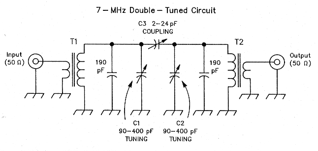
Fig 1 - A double-tuned-circuit filter for 40 m. Cl and C2 are mica-dielectric compression trimmers; C3 is an air-dielectric variable. (There is usually no justification for using a variable coupling capacitor in practical double-tuned circuits for frequencies of 30 MHz and lower; instead, use a fixed capacitor of the value required by the filter design. This filter's variable coupling capacitor varies the filter response to illustrate concepts discussed in this article.) The tuned windings of T1 and T2 consist of 17 turns of #22 enameled wire on T-50-6 toroidal, powdered-iron cores; the transformers' untuned links at first consisted of three turns of insulated wire but were later reduced to two turns. See text and Fig 2.
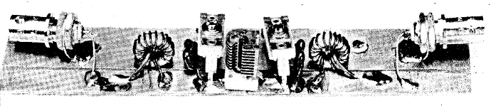
Fig 2 - An HF (7.1-MHz) double-tuned-circuit filter constructed for lab analysis.
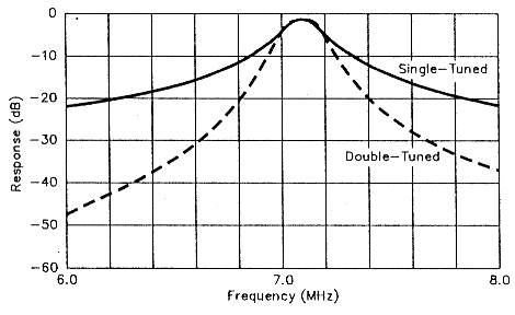
Fig 3 - Analysis of the filter shown in Figs 1 and 2. The solid curve shows the response of a single-tuned circuit; the dashed curve, a double-tuned circuit. Both filters are adjusted for maximum response at 7.1 MHz. The gap between the filterresponse maxima and the 0-dB line represents' the filters' insertion loss. (A computer generated the data for this and the other graphs in this article; experiment confirmed the data.)
I'll examine the fundamentals of the double-tuned circuit by describing the 40-m filter shown in Figs 1 and 2. Fig 3 graphs an analysis of the circuit. The solid-line plot shows gain versus frequency for a single-tuned circuit filter. The dashed plot shows the performance of a double-tuned circuit filter. Both filters are designed to be doublyterminated, with 50 Ω at input and output. Both have a 7.1-MHz center frequency and a 200-kHz bandwidth. The response magnitudes are similar for the single- and double-tuned circuits; their differences become significant only at frequencies removed from passband center in the filter stopband. We use double-tuned-circuit filters in place of single-tuned designs because double-tuned filters provide higher stopband attenuation.
The two tuned circuits shown in Fig 1 use toroidal transformers (T1 and T2) tuned with mica-dielectric compression trimmercapacitors (C1 and C2, TUNING). A 2-to-24 pF air-dielectric capacitor (C3, COUPLING) couples the resonators. Two-turn links provide input/output coupling to and from 50 Ω. (I originally used three-turn links; I'll describe later why I reduced them by one turn.)
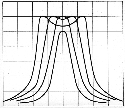
First, I set the COUPLING capacitor to maximum and adjusted the two TUNING capacitors for maximum response with the signal generator set to 7.1 MHz. Then I tuned the generator from 6 to 8 MHz to examine the filter's overall response. Fig 4 shows the result: an overcoupled filter response in which two peaks bound a region of increased attenuation.
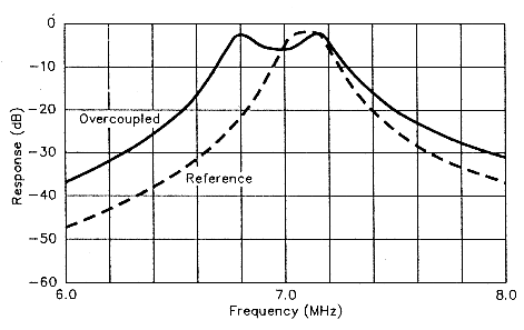
Fig 4 - Too much resonator coupling (in this example, too much capacitance at C3) overcouples the filter resonators and produces a two-peaked response. This is not caused by tuning the resonators to different frequencies. The reference plot shows the desired single-peak response.
This double-humped response is not the result of stagger tuning, that is, it's not caused by tuning the resonators to slightly different frequencies. Rather, both resonators are tuned to the same frequency. The peak amplitude of the double-humped response of Fig 4 is about the same as that of the desired filter, labeled REFERENCE.
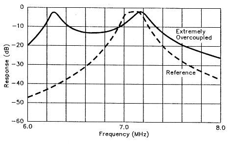
Fig 5 - Extreme overcoupling can produce two widely separated peaks, either of which can appear to an experimenter operating with limited test equipment to be the single sharp response of a properly adjusted filter. The reference plot shows the desired single-peak response.
Fig 5 is a more extreme example of over-coupling: I added capacitance across C3 tobring the coupling capacitance up to 65 pF. This moves the peaks even farther apart and increases the depth of the valley between them. This situation can be especially perplexing to the home experimenter because either peak may appear to be the single peak expected of the filter. This illustrates the importance of swept-frequency instrumentation in evaluating double-tuned circuits checking the filter response through a range of frequencies. You'll never notice an overcoupled double-tuned circuit's second peak if you merely adjust its resonators for maximum response at a single frequency!
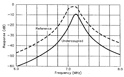
Fig 6 - Insufficient resonator coupling produces a too-sharp peak and abnormally high insertion loss. As in Figs 4 and 5 (and the Double-Tuned plot in Fig 3), the reference plot shows the desired filter response, the response obtained by critical coupling.
Fig 6 shows the other extreme, the under-coupled double-tuned circuit. I obtained this single, sharp peak by adjusting C3, COUPLING, to its minimum value (2 pF). This filter is too narrow; its insertion loss is excessive.
The desired double-tuned-circuit-filter response is usually critical coupling, shown by the reference plot in Figs 3 through 6. A critically coupled filter has only one peak, without excessive insertion loss. (I'll discuss the difference between excessive and proper insertion loss shortly.)
You can experimentally achieve critical coupling as follows: Set up the circuit for undercoupling and align the filter in this condition. Loss will be large. Increase coupling in small steps, readjusting the filter tuning capacitors and sweeping the filter response after each coupling increase. Continue this procedure until you observe double peaking. Slightly decrease the coupling from the double-peak value and measure the filter bandwidth.
This procedure produced a smooth, single, almost flat response in the experimental 40-m filter. Initially, however, the bandwidth was too wide (324 kHz), with an insertion loss of 1.2 dB. 1 reduced the transformers' three-turn links to two turns and repeated the process. The result: a critically coupled filter that's 178 kHz wide, with just over 2 dB of insertion loss.
Measuring Double-Tuned Circuit Performance
Simple, home-built instrumentation usually suffices for double-tuned-circuit adjustment at HF and VHF. The main parameter of interest is filter gain versus frequency; this can be measured with the test setup of Fig A.
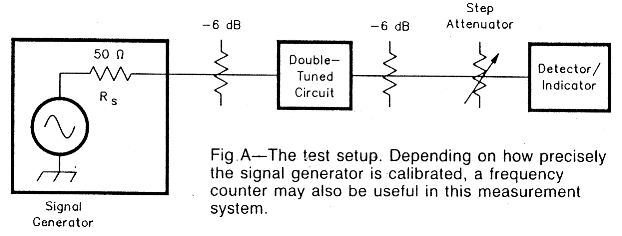
The first element is a signal source. I usually use home-brew generators at -HF and VHF, each with an available output of about 10 mW.(a),(b) Fixed attenuators in line with the input and output of the filter under test provide the filter with clean 50-Ω source and load terminations.
The next element is a step attenuator. This block is very fundamental; it becomes the cornerstone for a system for home RF measurements. I use surplus and home-brew attenuators.(c)
The final element is a sensitive detector. This can be a 50-Ω-terminated oscilloscope, a spectrum analyzer or even a simple power meter. I made all measurements reported in this article with the circuit shown in Fig B a microwatt meter consisting of a biased diode detector followed by an operational-amplifier meter driver. The detector is preceded by a two-stage amplifier using MMICs. The detector should be capable of responding to signals 30 to 60 dB weaker than the signal-generator output.
Begin your measurements with a calibration. Tune the generator to the frequency of interest and replace the filter with a direct coaxial connection between the fixed attenuators. Note the attenuator setting for a full-scale meter reading and record this in your notebook. Compare this figure with the peak-filter-response readings to determine insertion loss. Check'the system's calibration often, for levels often drift with time.
This test setup can also measure filter bandwidth. Align the filter and adjust the generator frequency for maximum response. Set the attenuator to provide a full-scale meter reading. Increase attenuation by 3 dB. Carefully note the new, lower meter reading. Reset the attenuation to the previous level, bringing the meter back to full scale. Then tune the signal generator, first to one side of the filter peak and then to the other, stopping in each case when the response equals the new, lower meter reading just described. The frequency difference between these points is the filter's - 3-dB bandwidth. - W7ZOI
- Solid-State Design for the Radio Amateur, p 170. See main-text note 1.
- W. Hayward, Beyond the Dipper, QST, May 1986, pp 14-20; Feedback, QST, Aug 1986, p 40.
- R. Shriner and P. Pagel ,A Step Attenuator-You Can pond, QST, Sep 1982, pp 11-13.
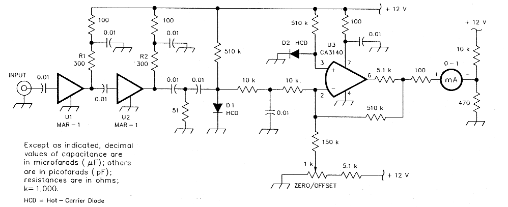
Fig B - A detector/indicator suitable for filter evaluation and alignment. All capacitors are disc-ceramic; all resistors are 1/4-W, carbon-film. D1 and D2 are hot-carrier diodes (HP.5082-2672, 1N5711 or equivalent). 1.11 and U2, shown as Mini Circuits MAR-1 MMICs, can be directly replaced with Avantek MSA-0185 MMICs, or, if you use 270-0 resistors at R1_ and R2 instead of the 300-0 resistors shown, with Motorola MWA-120 MMICs. Adjust the ZERO/OFFSET control for a meter indication of 0 with no RF present.
A VHF Double-Tuned Circuit
The double-tuned circuit and the adjustment methods just described can easily be applied at higher frequencies. 1 needed a filter for a 2-m SSB transceiver's receive and transmit signal paths, a filter no wider than about 2 MHz to attenuate the image frequency (124 MHz in my application) by 50 dB. The filter I constructed becomes our second example.
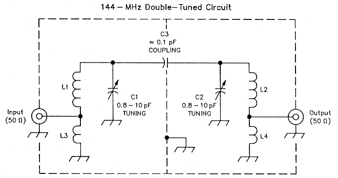
Fig 7 - This VHF double-tuned circuit differs electrically from its HF relative (Fig 1) only in the means used to couple the filter ports to 50 Ω. The HF filter used small inductive links; this filter uses the autotransformer action of L1-L3 and L2-L4, in effect, tapped coils. Cl and C2 are 0.8- to 10-pF air-dielectric piston trimmers (Johanson); standard air-dielectric variables are also suitable. C3 is a wire probe, soldered at only one end (the Cl-L1 junction in this case; it doesn't matter which) that passes through a hole in the filter shield partition for electrostatic coupling to the C2-L2 junction. L1 and L2 each consist of 7 turns of #14 tinned copper wire, 1/4-inch inner diameter. L3 and L4 each consist of approximately 0.6 inch of #18 tinned copper wire. Fig 8 shows three filters constructed in this way.
Fig 7 shows the VHF-filter topology I used. Each resonator consists of two inductors. L1 and L2 contribute most of the resonator inductance; L3 and L4 are end-loading elements consisting of small lengths of #18 wire connected to circuit common. Coaxial connectors attach to the L1-L3 and L2-L4 junctions. I find this topology easier to adjust than taps on a coil.
The filter is built on a scrap of circuit-board material. Vertical walls serve as shield sections for each resonator and provide for component mounting. You may not need to add a lid if the walls extend well above the board (perhaps 1.5 inches or more) and if you mount the components close to the board. A lid is mandatory, even during adjustment, if the walls are short.
A very low-value adjustable capacitor (C3 in Fig 7, illustrated by the three examples in Fig 8), couples the filter sections. C3 consists of a piece of plastic-insulated wire that's soldered to one of the tuning capacitors, routed through a hole in the shield partition and placed in proximity to the other tuning capacitor.
The partition is necessary; it eliminates stray coupling between filter elements, a fact confirmable through measurement.
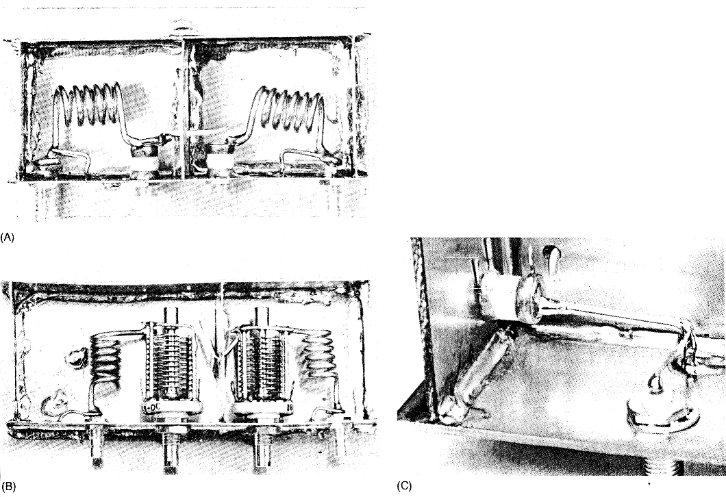
Fig 8 - Two VHF (A and B, for 2 m) and one UHF (C) doubletuned-circuit filters. The filter at A uses piston air-dielectric trimmers (Johanson); at B, standard air-dielectric trimmers (in this case, split-stator butterfly units with stators paralleled). Piston trimmers afford more precise adjustment and higher Q. C details one section of a 70-cm filter in which each resonator inductor (L1-L3 and L2-L4 in Fig 7) consists entirely of an L-shaped length of #14 tinned wire, the end-loading inductor (L2 or L4 in Fig 7) being the short section between the elbow and ground. In each filter, the coupling capacitor (C3 in Fig 7) consists of a wire probe that passes through the shield partition. Adjusting the wire's length (and the proximity of its unconnected end to the tuned circuit it probes) varies filter coupling.
Filter shielding, including an inter-resonator partition, is essential at VHF/UHF because even stray capacitance can overcouple a filter. Solenoidal resonators must be shielded for an additional reason: Unlike toroidal coils, they can couple to each other and associated circuitry via their external magnetic fields.
Double-Tuned Circuits; Not Necessarily Top-Coupled
Radio technologists sometimes characterize the Fig 1 , and Fig 7 circuits as top-coupled because capacitance between the tops (ungrounded ends) of their resonators couples the filter sections. Top-coupled double-tuned circuits are common; one popular QST project(d) uses them in its RF-amplifier circuitry, for instance. The relative commonness of this special case of the double-tunedcircuit leads some experimenters to conclude that double- tuned circuit necessarily implies two top-coupled circuits. But this is not so.
Coupling two circuits together merely means that energy from one circuit somehow gets into the other; such coupling can be inductive, capacitive or, both; top; bottom,. or both (Fig A), What matters. more is that.whatever coupling exists allows you to achieve the filter response you seek, and that whatever unwanted or stray coupling` exists doesn't compromise that response--in the filter's passband and stopband over the frequency range of interest, Predictable, repeatable filters minimize coupling somehow through builder and designer know-how. -David Newkirk, WJ1Z
- W. Hayward and J. Lawson, A Progressive Communications Receiver, QST, Nov 1981, pp 11-21; Feedback; 1982 QST: p 47, Jan; p 54, April, p 41, Oct; also in the ARRL Handbook (1982 through present editions).
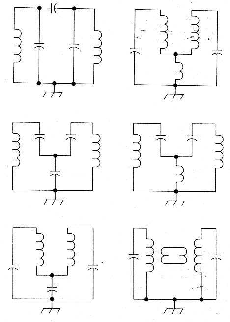
Fig A - Double-tuned circuits can be coupled inductively, capacitively or both; top, bottom or both. These examples show only a few of the possible combinations. Sometimes the mere proximity of circuit components suffices; see Fig B.
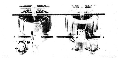
Fig B - ARRL Lab Engineer Zack Lau, KH6CP, who lives 1 mile from W1AW, originally built this undercoupled double-tuned filter to knock down W1AW at 3581.5 kHz during QRP contests centering at 3560 kHz. Now reconfigured for 75-m SSB, the filter specs out like this: -3-dB bandwidth, 8 kHz; -60-dB bandwidth, 310 kHz; insertion loss, 21 dB. Each coil consists of 17 turns of #16 wire on a T-200-6 toroidal, powdered-iron core (Qu= 482 at 3.8 MHz). The tuning capacitor in each section consists of paralleled 56-pF silver-mica, 240-pF chip and 2- to 19.3-pF air-dielectric capacitors. Silver-mica end-loading capacitors (10 pF, between each resonator top, and the BNC jacks) couple the filter to 50-Ω reality.
The resonators are exactly 1 inch apart, core to core (the spacing is adjustable). Can we accurately calculate the tiny capacitance between them? Should we characterize this filter as capacitively top-coupled? Maybe what matters more is that using this filter on a band where you usually kick in a 20-dB attenuator anyway also makes your receiver front end 8 kHz wide!
(Likewise, the outer walls prevent coupling between the filter elements and external circuitry.) In one version of this filter with 0.7-inch-high shield walls, enough stray coupling existed to produce a severely over-coupled response with C3 (the probe wire) absent! The coupling disappeared when I placed a lid over the two compartments. Good lid-to-wall electrical contact is mandatory; I used C clamps during alignment. Eventually, I'll solder a lid in place.
VHF/UHF double-tuned circuit adjustment resembles the procedure I describedfor the 7-MHz example. Install a longerthan-necessary coupling wire and bend it close to the probed resonator's hot (ungrounded) end. Tune the filter and sweep its response. You should observe a double-humped response. If you can't find two peaks, increase the coupling until you do. Once you observe overcoupling, decrease coupling by reducing the wire length or changing its position. Then measure the filter's bandwidth and insertion loss. The bandwidth probably won't be right at first; you can set the filter's band-width by adjusting the end-loading inductors (L2 and L4) and adjusting the coupling after each loading change.
The 2-m filter performs as expected, exhibiting a bandwidth of about 2 MHz and an insertion loss of 3 dB. (A similar filter I built uses #18 wire instead of #14 wire for the main inductors. Although I can adjust it to obtain a 2-MHz bandwidth, its insertion loss exceeds 6 dB.)
How Narrow is Narrow?
Experiments like these clearly indicate a relationship between filter selectivity and insertion loss. Loss is also related to the components' unloaded Q (Qu). The parameter Qo (normalized Q) summarizes these dependencies. Qo is defined as the ratio Qu/Qr, where Qu is unloaded resonator (inductor) Q and Q f is the filter Q, which equals filter center frequency divided by filter bandwidth. Fig 9 graphs filter insertion loss versus normalized Q.(2)
The 40-m filter of Fig 1 has a design bandwidth of 200 kHz hence, a Qt of 7/0.2, or 35. Building this filter using resonators with an unloaded Q of 250 results in a normalized Q of 250/35, or 7.1. The Fig 9 curve shows an insertion loss of about 2 dB for Qo = 7; this agrees with my measurements.
Fig 9 also shows that insertion loss becomes very large for normalized Qs of less than 2. As a reasonable limit, doubletuned-circuit filter Q should be no more than about 40% of the unloaded resonator Q.
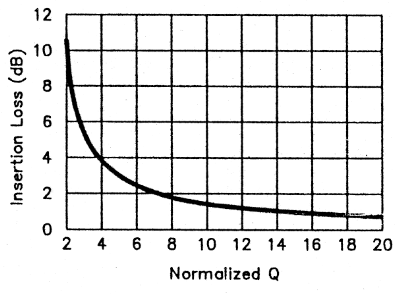
Fig 9 - Double-tuned-circuit insertion loss versus normalized 0, Qo (unloaded Q [Qu divided by filter Q [Qt]). Higher insertion loss accompanies narrower bandwidths; a reasonable limit for the double-tuned circuit is Qo > 2.5.
Summary and Additional Thoughts
The double-tuned circuit can be summarized as follows:
- Double-tuned circuits can be characterized by degree of coupling. A circuit may be undercoupled, overcoupled or critically coupled.
- A double-humped response indicates overcoupling, and rarely has anything to do with stagger tuning.
- An experimenter may overlook the other peak in a severely overcoupled circuit because it may be far Femoved in frequency from the observed peak. Builders should take special care to avoid mistaking one of two peaks as the single peak of a critically coupled circuit.
- Align double-tuned circuits by adjusting their coupling from slight overcoupling toward critical coupling. You should observe slight overcoupling during the alignment process.
- Higher insertion loss accompanies narrower bandwidths. A reasonable limit for the double-tuned circuit is Qo > 2.5. All of the concepts governing the double-tuned circuit may be extended to filters of other orders. For example, a single-tuned circuit has an insertion loss related to bandwidth and unloaded Q. Similar relations exist for filters consisting of multiple coupled resonators. Crystal filters, arrays of dielectric resonators, and coupled microstrip sections all behave similarly. They can all be tuned with these methods.
Notes
- W. Hayward and D. DeMaw, Solid-State Design for the Radio Amateur, Appendix 2, Band-pass filters, p 239 (Newington: ARRL, 1986). Also see W. Sabin, Designing Narrow Band-Pass Filters with a BASIC Program, QST, May 1983, pp 23-29.
- Insertion loss (dB) = 20 log (Qo / (Qo - 1.414))
W7ZOI, Wes Hayward