Simple RF-power measurement
Making power measurements from nanowatts to 100 watts is easy with these simple homebrewed instruments!
Measuring RF power is central to almost everything that we do as radio amateurs and experimenters. Those applications range from simply measuring the power output of our transmitters to our workbench experimentations that call for measuring the LO power applied to the mixers within our receivers. Even our receiver S meters are power indicators. The power-measuring system described here is based on a recently introduced IC from Analog Devices: the AD8307. The core of this system is a battery operated instrument that allows us to directly measure signals of over 20 mW (+13 dBm) to less than 0.1 nW (-70 dBm). A tap circuit supplements the power meter, extending the upper limit by 40 dB, allowing measurement of up to 100 W (+50 dBm).
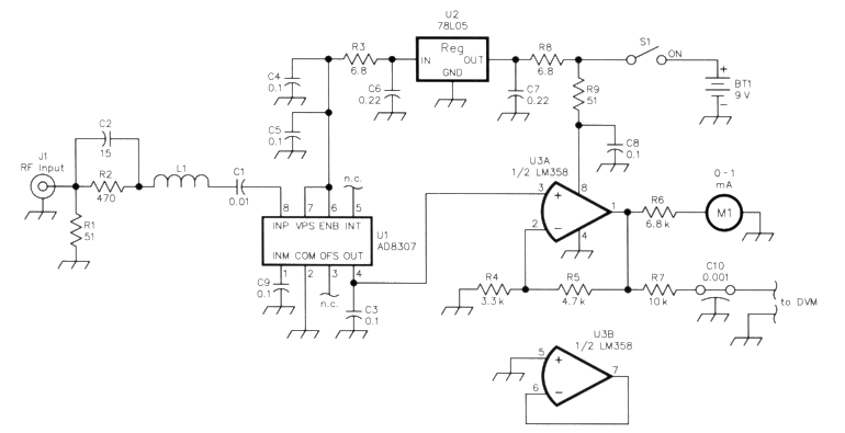
Figure 1 - Schematic of the 11- to 500-MHz wattmeter. Unless otherwise specified, resistors are 1/4-W 5%-tolerance carbon-composition or metal-film units. Equivalent parts can be substituted; n.c. Indicates no connection. Most parts are available from Kanga US(2).
| J1 - N or BNC connector L1 - 1 turn of a C1 lead, 3/18 inch ID; see text. M1 - 0-15 V dc; see text. |
S1 - SPST toggle U1 - AD8307(1) U2 - 78L05 U3 - LM358 |
Misc: See Note 2; copper-clad board, enclosure |
The power meter
The cornerstone of the power-meter circuit shown in figure 1 is an Analog Devices AD8307AN logarithmic amplifier IC, U1. Although you might consider the IC as slightly expensive at about $10 in single quantities, its cost is justified by the wide dynamic range and outstanding accuracy offered. You can order the part directly from the Analog Devices Web site, which also offers a device data sheet.(1)(2)
U1's power supply can range from 2.7 to 5.5 V. A 5-V regulator, U2, provides stable power for U1. U3, an opamp serving as a meter driver completes the circuit. U1's dc output (pin 4) changes by 25 mV for each decibel change in input signal. The dc output is filtered by a 0.1 µF capacitor and applied to the noninverting input of U3, which is set for a voltage gain of 2.4. The resulting signal with a 60 mV/dB slope is then applied to a l mA meter movement through a 6.8 kΩ multiplier resistor. When the circuit is driven at the 10-mW level, U3's output is about 6 V. U3's gain-setting resistors are chosen to protect the meter against possible damage from excessive drive.U1 has a low-frequency input resistance of 1.1 kΩ. This combines with the resistances of R1 and R2 to generate a 50 Ω input for the overall circuit. R2 in parallel with C2 form a high-pass network that flattens the response through 200 MHz. Ll, a small loop of wire made from a lead of C1, modifies the low-pass filtering related to the IC input capacitance, extending the response to over 500 MHz.
M1 is a RadioShack dc voltmeter. Although sold as a voltmeter, it actually is a 0 - 1 mA meter movement supplied with an external 15 - kΩ multiplier resistor. The 0 to 15 V scale is used with a calibration curve that is taped to the back of the instrument to provide output readings in dBm. The dBm units can be converted to milliwatts by using a simple formula, although dBm readout is generally more useful and convenient.(3)
An auxiliary output from C1O, a feedthrough capacitor, is provided for use with an external digital voltmeter or an oscilloscope for swept measurements.(4) We use the DVM when resolution is important. The analog movement can be read to about 1 dB, which is useful when adjusting or tuning a circuit. Enterprising builders might program a PIC processor to drive a digital display with a direct reading in dBm.
The first power meter we built did not include R2, C2 and L1. That instrument was accurate in the HF spectrum and useful beyond. Adding the compensation components produced an almost flat response extending beyond 500 MHz with an error of only 0.5 dB. The compensation network reduces the sensitivity by about 3 dB at HF, but boosts it at UHF. If your only interest is in the HF and low VHF spectrum through 50 MHz, you can simplify the input circuit by omitting R2, C2 and L1. The responses before and after compensation are shown in figure 2.
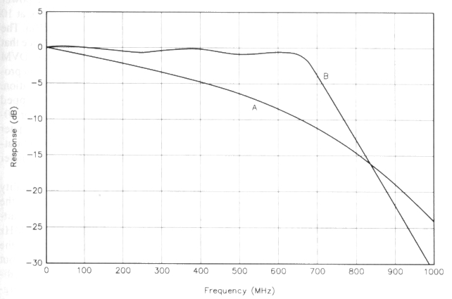
Figure 2 - Response curves for the power meter before (A) and after (B) addition of R2, C2 and L1.
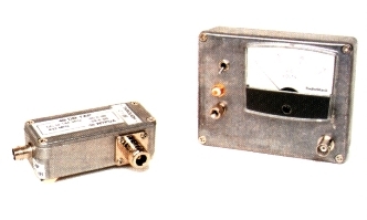
The power meter is constructed "dead-bug" fashion without need of a PC board. It is breadboarded on a strip of copper, clad PC-board material held in place by the BNC input connector. R1 is soldered between the center pin and ground with short leads. U1 is placed abou t 3 /4 inch from the input in dead-bug fashion (leads up) with pins 1 and 8 oriented toward J1. The IC is held to the ground foil by grounded pin 2 and bypass capacitors C3, C4 and C5. R2 and C2 are connected to the J1 center pin with short leads. L1 is formed by bending the lead of C1 in a full loop. Use a 3/16 inch diameter drill bit as a winding form. None of the remaining circuitry is critical. It is important to mount the power meter components in a shielded box. We used a Hammond 1590BB enclosure for one meter and a RadioShack box for the other, with good shielding afforded by both. Don't use a plastic enclosurefor an instrument of this sensitivity.
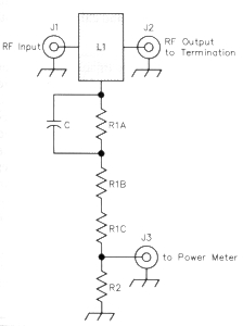 |
Figure 3 - A tap that attenuates a highpower signal for use with the power meter. See the text and Figure 4 for discussion of the capacitor, C. J1, J2 - N connectors; see text. J3 - BNC connector L1 - 1 × 1/2-inch piece of sheet brass; see text. R1A - R1C - Three series-connected, 820 Ω, 1/2-W carbon film R2 - 51 Ω, 1/4-W carbon film |
Higher power
Transmitter powers are rarely as low as the maximum that can be measured with this power meter. Several circuits can be used to extend the range including the familiar attenuator. Perhaps the simplest is a resistive tap, shown in figure 3. This circuit consists of a flat piece of metal, L1, soldered between coaxial connectors J1 and J2 , allowing a transmitter to drive a 50 Ω termination. A resistor, Rl, taps the path to route a sample of the signal to J3, which connects to the power meter. R2 shunts J3, guaranteeing a 50 Ω output impedance. Selecting the values that comprise R1 establishes the attenuation level.
The tap extends the nominal + 10 dBm power meter maximum level to +50 dBm, or 100 W. Power dissipation becomes an issue at this level, so Rl is built from three series -connected half-watt, carbonfilm resistors.
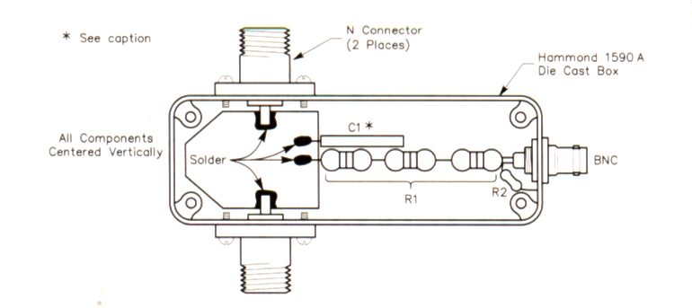
Figure 4 - Drawing of the 40-dB power tap assembly shown schematically In Figure 3. The center conductors of the two N connectors (RF INPUT and RF OUTPUT) are connected by a 1 x 1/2 inch place of sheet brass with Its corners removed to clear the pillars. In the Hammond 1590A die-cast aluminum enclosure. C1 Is made from a piece of #22 AWG Insulated hook-up wire; it extends 0.6 inch beyond the edge of the tinned metal piece and almost rests against the two resistor bodies.
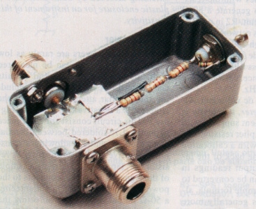
An inside view of the simple attenuator shown in figure 3.
The tap is built with the J1 to J2 connection configured as a 5042 transmission line as shown in figure 4 and the accompanying photographs. Adjustments were performed with an HP-8714B network analyzer. The analyzer was used to adjust the value of C for an attenuated path to J3 that is flat within 0. 1 dB up to 500 MHz. The tap can then be used with a spectrum analyzer or laboratory grade power meter.
It is not realistic to achieve 0.1-dB accuracy through UHF without a network analyzer for adjustment. However, if the tap is duplicated using the mechanical arrangement of figure 4, you can expect the tap to be flat within about 1 dB through 500 MHz. The low-frequency attenuation is determined merely by the resistors, so can be guaranteed with DVM measurements. If the primary interest is in measurements below 150 MHz, you can replace the N connectors with BNC connectors. The tap is housed in a Hammond 1590A box.
Calibration
We read and use our meters in one of two ways. The DVM output is recorded and used with an equation that provides power in dBm. Alternatively, we read the panel meter and look at a chart taped to the back of the instrument. In both cases, we need a known source of RF power to calibrate the tool.
The easiest way to calibrate this instrument is with a calibrated signal generator. Set the generator for a welldefined output and apply it to the power meter. We did our calibration work at 10 MHz and levels of -20 and -30 dBm. The two levels provide a 10-dB difference that establishes the slope in decibels per DVM millivolt. One of the two values then provides the needed constant for an equation. The signal generator can be stepped through the amplitude range in 5- or 10- dB steps to generate data for the meter plot. figure 5 shows a plot of DVM output Vs power meter reading. The meter plot is similar.
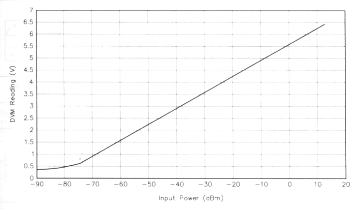
Figure 5 - Plot of the DVM output versus generator power.
If you don't have access to a quality signal generator, you can calibrate the power meter using a low-power transmitter. A power level of 1 to 2 W at 7 MHz is fine. Attach the transmitter through the tap to a dummy load where the output voltage can be read directly using a diode detector and DVM as shown in Figure 6. If the power output is 1 W, the peak RF voltage will be 10 V. The detector output will then be about 9.5 V and the signal to the power meter is -10 dBm. Adding a 10-dB pad, as shown in Figure 6, at the meter input drops the power to -20 dBm for the second calibration point.
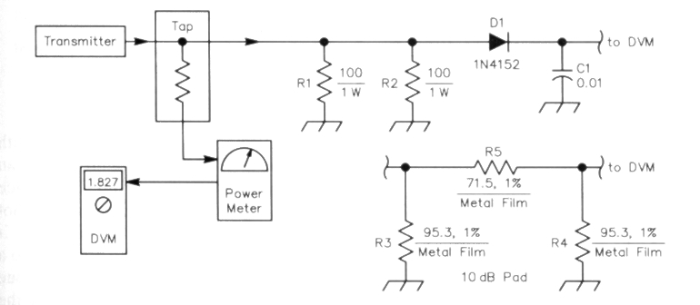
Figure 6 - If a signal generator Is not available, calibration can be done using a lowpower transmitter. Resistor values for a 10-dB pad are shown.
| C1 - 0.01 µF disc ceramic D1 - 1N4152 R1, R2 - 100 Ω, 1 W |
R3, R4-95.3 Ω 1% metal film R5 - 71.5 Ω, 1% metal film |
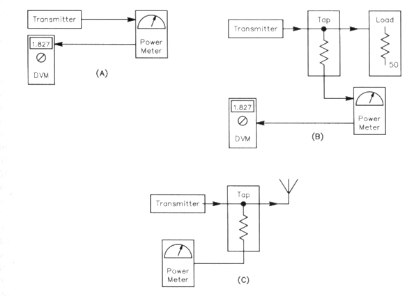
Figure 7 - Power measurement schemes for various situations; see text for an explanation.
Applications
There are dozens of applications for this little power meter, a few of which are shown in the accompanying figures. Some applications are obvious and practical while others are more elaborate and instructive. Most of these measurements are substitutional, where the power meter is substituted for a load in a circuit. In contrast, most measurements with an oscilloscope are in situ, performed in place within a working circuit.
Figure 7A shows power measurement for early stages of a transmitter, very low power transmitters, or signals from other sources. Among the most common is measurement of the power available from a LO system that will then drive a diodering mixer. The nominal maximum power or the meter is + 13 to + 16 dBm. We were able to perform measurements nearly up to +18 dBm at HF, but this is not maintained at the VHF. Careful calibration at HF was made by comparing our meters outputs to those of an HP435A.
The tap of figure 3 extends transmitter testing with the setup of figure 7B. A good dummy load (termination) is placed on the tap output with the transmitter attached to the input. The power in dBm is now that read on the meter in dBrn plus the tap attenuation in decibels.
We sometimes wish to measure power during an operating session. This can be done with the setup of figure 7C. A typical application might be a QRP station where the operator experiments with significantly reduced, but variable power.
The power meter is useful for a variety of applications with bridge circuits. Figure 8 shows the meter as the detector for a return loss bridge (RLB) driven by a signal generator.(5) In this example, we use the system to adjust an antenna tuner. Because of the excellent sensitivity of the power meter, the generator need not have high output power. For example, we often make these measurements with a homebrew generator delivering +3 to + 10 dBm.
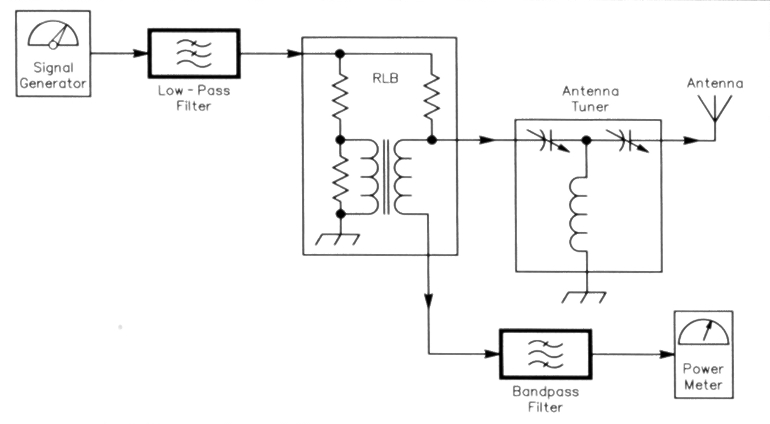
Figure 8 - Using the power meter for bridge measurements
The use of such low power can complicate the measurements, as we discovered when we tried the experiment of figure 8. The exercise began without either of the filters shown. When the generator was turned on, the power meter indicated -4 dBm from the RLB. We tune the matching circuit, but could only achieve -25 dBm, indicating 21 dB return loss.(6) No further improvement could be observed. This was the result of local VHF TV and FM broadcast interference. A bandpass or low-pass filter in the power-meter input eliminated the residual response, allowing us to achieve a 45-dB return loss with further tuning. But this was also a limit where no further improvement seemed possible. Adding a low-pass filter to the signal generator output reduced the harmonics there, allowing further improvement. We were eventually able to tune the system for an absurd 60 dB return loss (SWR = 1.002), generally impossible to measure with normal bridges using diode detectors.
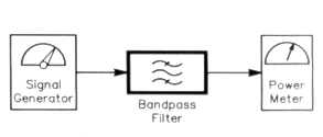
Figure 9 - Filter measurements with the power meter.
The power meter is ideal for experiments with various RF filters as shown in figure 9. A signal generator is attached to the filter input with the power meter terminating the output. The filter may then be tuned or swept. Temporarily replacing the filter with a coaxial through connection allows you to evaluate filter insertion loss. Both the power meter and the signal generator are 50 Ω instruments, so the filter will need matching networks if it is not a 50 Ω design.
As with the previous example, measurement anomalies can be observed when investigating filters. For example, after using the power meter to adjust a 7 MHz bandpass filter we were able to easily measure the second-harmonic content of the signal generator when tuned to 3.5 MHz.
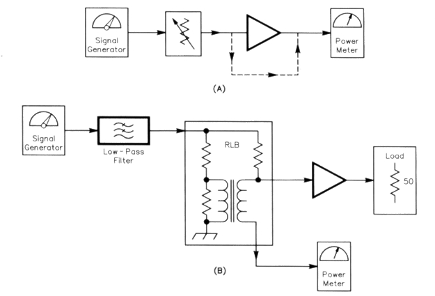
Figure 10 - Amplifler measurements with the power meter. At A, making gain measurements. At B, a method to determine the Input-impedance match. Reversing the amplifier terminals allows investigating reverse gain and output match
Figure 10A shows the power meter used with a signal generator to study amplifier circuits. A step attenuator is shown with the generator, allowing the power level to be reduced while preserving a 50 Ω environment. Generally, a drive level of -30 dBrn is low enough with typical circuits. The system is initially set up with a through connection, indicated by the dotted line. Then the amplifier is inserted and the output power is measured. The difference between the two responses, each in dBm, is the gain in decibels. An interesting and easily performed related measurement is that of amplifier reverse gain. Merely swap the amplifier terminals, attaching the generator to the output and the power meter to the input. The measured gain will now be a negative decibel number.
Amplifier investigation continues with the setup of figure 10B where we use an RLB to measure the input impedance match. Although a simple bridge will not provide the actual input impedance, it will tell you how close the circuit is to a perfect match. Adjustments can be done to achieve a match. Again, reversing the amplifier allows examining the output. We included a low-pass filter in the generator output, a precaution that may also be useful with the gain-determination setup. The measurements of figure 10 provide the information normally provided by a scalar network analyzer.
The power meter can serve as the detector for a number of simple instruments. Figure 11 shows a simple RF sniffer probe, handy for examining circuit operation. The probe consists of a small inductor attached to the end of a piece of coaxial cable (RG-58, RG-174, or similar). A few ferrite beads of about any type are placed over the outside of the cable near the coil. The probe can be placed close to an operating circuit to look for RF. The smaller the link diameter, the greater the spatial resolution can be. This is a scheme that actually lets you see selfoscillation in an amplifier, much more useful than a speculation that a circuit "might be oscillating."
The power meter can be used with other probes. One might be a simple antenna that would allow field-strength determinations. Another is a resonance- indicating probe that would provide traditional dip meterlike measurements, but with improved accuracy and sensitivity.(7)
A recent QST project developed by Rick Littlefield, K1BQT, uses anAD8307 as a relative RF indicator.(8) That instrument, with the probe described in the sidebar by Ed Hare, W1RFl, is aimed at examining conducted electromagnetic interference (EMI). Our power meter should function well with that probe. There is great potential for small portable instruments for the study of both conducted and radiated EMI.
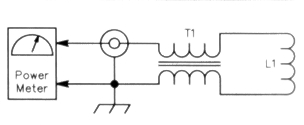
Figure 11 - An RF sniffer probe that alows observation of relative RF levels. This probe allows you to see selfoscillation In amplifiers, or proportional responses in a receiver or transmitter.
L1 - Two turns of insulated wire, 1/4 inch ID.
T1 - Several ferrite beads on a length of coaxial cable; see text.
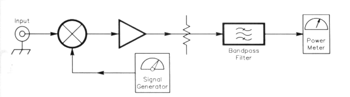
Figure 12 - Adding a few components to a signal generator and the power meter creates a measurement receiver. The kinds of measurements possible depend on the filter used. See the text for some possibilities.
Figure 12 shows an example of some simple instruments that can be built using the power meter as a foundation. Here, the signal generator becomes the LO for a mixer such as the popular diode ring. This drives an optional amplifier and attenuator, followed by a bandpass filter. The power meter measures the filter output. The result is a custom measurement receiver.
We have built two variations of this project. The first uses a three-resonator LC bandpass filter tuned to 110 MHz, while the signal generator tunes from 50 to 250 MHz.(9) A Mini-Circuits MAV-11 is used for the amplifier. The resulting receiver can then be used to measure signals over the entire spectrum up to 360 MHz with sufficient resolution to examine transmitter spurious responses.
The second measurement receiver uses a homebrew 5-MHz crystal filter with a 250-Hz bandwidth. The signal generator is a homebrew unit with extreme tuning resolution, or bandspread. This instrument was used to measure SSB-transmitter carrier and sideband suppression and IMD, and for examining spurious output of experimental frequency synthesizers.
Concluding thoughts
The traditional view of a power meter is as an instrument that examines transmitter output. But it can be much more than that. The AD8307 allows you to build a power meter that turns a common Amateur Radio station into the beginnings of a RF measurement lab.
Our thanks to Barrie Gilbert of Analog Devices Northwest Labs for providing the AD3807 IC samples.
Notes
- https://www.analog.com/en/index.html. The data sheet includes an extensive discussion of the theory of operation of the logarithmic detector and applications beyond the scope of this article.
- PmW = 10^dBm/10
- Feedthrough capacitors are available from Down East Microwave Inc, 954 Rt 519, Frenchtown, NJ 08825; tel 908-996-3584, fax 908-996-3702; https://www.downeastmicrowave.com/Default.asp.
- See Wes Hayward, W7ZOI, and Doug DeMaw, W1 FB, "Solid-State Design for the Radio Amateur," p 154, ARRL, 1977. Directional couplers are also useful in this application, such as that used in the classic W7EL power meter, Roy Lewallen, W7EL, "A Simple and Accurate QRP Directional Wattmeter," QST, Feb 1990, pp 19-23 and 36.
- A return loss of 21 dB corresponds to a SWR of 1.196, already a great match for most practical antenna situations.
- See Wes Hayward, W7ZOI, "Beyond the Dipper," QST, May, 1986, pp 14-20. Also, the signal-generating portion of that instrument is useful as a simple, general-purpose RF source.
- Rick Littlefield, K1BOT, "A Wide-Range RF-Survey Meter," QST, Aug 2000, pp 42-44; see also Feedback, Oct 2000, p 53.
- Wes Hayward, W7ZOI,"Extending the Double-Tuned Circuit to Three Resonators," QEX, Mar/Apr 1998, pp 41-46. The band-pass filter was then used in the instrument described in
- Wes Hayward, W7ZOI, and Terry White, K7TAU, "A Spectrum Analyzer for the Radio Amateur," QST, Aug 1998, pp 35-43; Part 2, Sep 1998, pp 37-40.
W7ZOI: w7zoi@easystreet.com
W7PUA: boblark@proaxis.com