Simplified design of impedance-matching networks 2
Pi and T Networks
In this second part it is shown how pi and T networks can be formed quite simply from the basic L network discussed in Part 1.
The L section has the advantages of great simplicity and optimum efficiency, but it is an inflexible arrangement in that only one set of constants will give the required match. The circuit Q, for example, cannot be chosen at will because it is fixed by the ratio of the two resistances. When an amplifier tube is being matched to a load, it is often just as important to have the proper operating Q in the tank as it is to have the proper loading.(6) Also, there are cases where the presence of reactance in the load makes it desirable to use a more complex network.
Two L sections can be combined to form either a pi or T network. Both the pi and T are useful arrangements for increasing the circuit Q and thus improving selectivity, and for increasing flexibility in adjustment.
The design methods used for these - or any other - combinations are practically identical. Basically there is just one method - the one used for designing the L section.
The Pi Network
Of all the possible configurations, the pi network is probably the one most familiar to amateurs because of its application as the tank circuit in r.f. power amplifiers. It lends itself to simple design methods when it is considered as two "back-to-back" L networks constructed to match an assumed "virtual" resistance at the meeting point.(7)
The principle is shown in Fig. 7. RP1 is the load (power-receiving device) to be matched to the source of power, which requires a load RP2. RP1 is the parallel resistance of the L section consisting of XP1 and -XS1, while R is the virtual resistance and corresponds to Rs in the circuits discussed in Part 1. Using R as the load, a second L section is formed by -XS2 and XP2 to transform R to the desired value of resistance for the power source to see. Each section is calculated separately by exactly the method described previously. The virtual resistance R must be smaller than either RP1 or RP2, since it is in the series arm of each section, but aside from this may be chosen at will or determined from other circuit requirements. The principal one of such requirements, in the case of an r.f. amplifier tank circuit, will be the desired operating Q.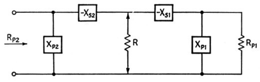
Fig. 7. Development of the pi network from two back-to-back L networks.
The design of such a circuit may be shown by continuing with the same resistance values used in the earlier example: a 52-ohm resistive load and a tube requiring a load of 2000 ohms. Let us now impose the requirement that the tank Q (Q2) be 12. From Equation 2B,
![]()
and from Equation 3A,
![]()
This is smaller than either of the two resistances being matched, and so is a proper value. Using Equation 3B, XS2 = 12 × 13.8 = 166 ohms. This completes the design of the L section on the input side of the network. Note that since Q2 is greater than 10, XP2 and XS2 are practically equal (although they must be of opposite types), which simply means that this much of the network is identical with an ordinary parallel-resonant tank circuit of the same operating Q.
We can now find the required Q (Q1) in the output section, since R and RP1 are known. Their ratio is 52/13.8 = 3.77, so from Equation 5 the required Q is
![]()
The same result could be found from Fig. 3. From Equation 3B, XS2 = 1,66 × 13,8 = 23 ohm and from Equation 2B,
![]()
The network design is now complete and is shown in Fig. 8A. The virtual resistance does not actually appear in the circuit, of course, so XS1 and XS2 can be added together and only one physical component is required. In this example it has a reactance of 166 + 23 = 189 ohms. The minus sign in Fig. 8A is used only to indicate that the reactance is of the opposite type to that chosen for XP1 and XP2.(8)
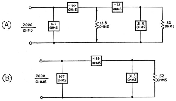
Fig. 8. Combining L-section elements into the pi configuration.
Reactance combinations
The design so far is quite general and we are free to choose types of reactance as we please, within the restriction that opposite types must be used in the two arms of each L section. There are four possibilities, as shown in Fig. 9, each leading to a different-looking final circuit but all providing the proper match between the two resistances. Fig. 9A is the best one for matching a tube to its load because it utilizes the components to best advantage in suppressing harmonics. Fig. 9B is a high-pass configuration and would be undesirable in a tank circuit. Note that in C and D the reactance of the connecting element in the practical circuit at the right is the difference between the reactances of the two series elements of the individual L sections, since opposite kinds of reactance are used in the series elements in these two cases.
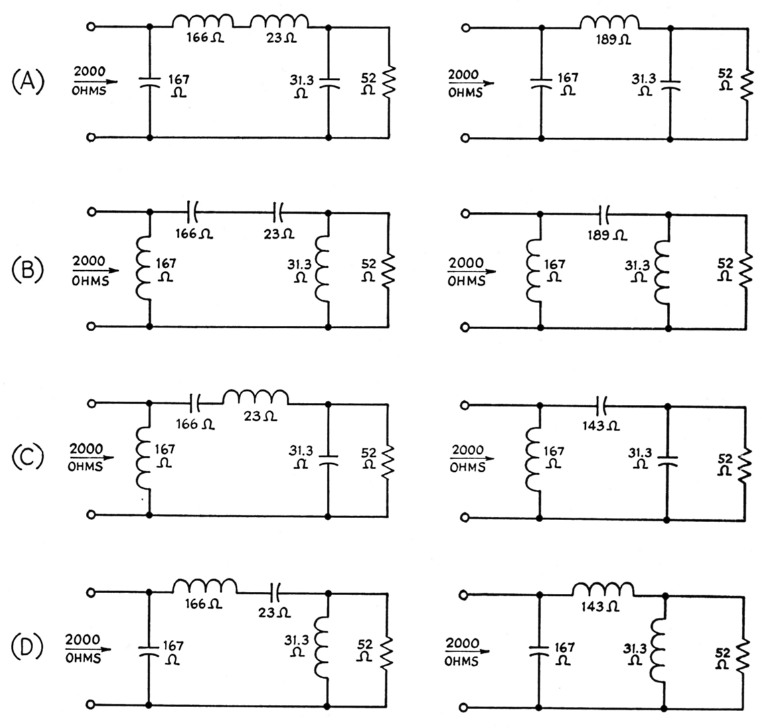
Fig. 9. The four possible combinations of L-sections into pi networks. Drawings at the left show the basic L sections; those at the right show the final forms.
The four circuits are shown primarily to illustrate the variety of networks, all of different appearance in the final version, that can be formed from simple L sections having fundamentally the same constants. They are alike only in that each will match 52 ohms to 2000 ohms. In other respects, such as relative suppression of frequencies higher and lower than the operating frequency, they are not identical. In some applications one or another of them might be preferable to Fig. 9A, but a decision cannot be made on this point until the nature of the problem is known.
Summary of pi network design
- Break the proposed network into two L sections as shown in Fig. 7.
- If the input section is to have a specified value of Q, use Equation 3A to find R. The value of R must be smaller than either of the two resistances to be matched. If it is not, a higher value of Q must be used.
- Or, if there are no restrictions on the Q of the input section, select some value for R that is less than either of the two resistances to be matched.
- Calculate the constants of the input L section to match the desired resistance, RP2, to R.
- Calculate the constants of the output section to match R to the other desired resistance, RP1.
- Add the values of the reactances in the series arms of the L sections (XS1 and XS2) to find the value of the series reactance in the pi network.
- Convert the final reactance values to inductance and capacitance.
Covering a band
The reactance values obtained from the design method apply at any frequency, so it is a simple matter to determine the range of variation that must be supplied to cover an amateur band. For example, using Equations 7 and 8 with the right-hand circuit of Fig. 9A for 3500 and 4000 kc. will give the following values for L and C:
| Reactance | 3500 kc. | 4000 kc. |
|---|---|---|
| 31.3 ohms (C) | 1450 pF | 1270 pF |
| 167 ohms (C) | 272 pF | 238 pF |
| 189 ohms (L) | 8.57 µH | 7.5 µH |
Note that all three tuning elements must be continuously variable within these limits to produce a match at any frequency in the band while maintaining a constant Q of 12.
Only two elements need be continuously variable to give a match if the consequent variation in Q is permissible. In this event the network should be designed for a minimum value of Q. It is convenient to use a fixed value of inductance and adjust the capacitances to achieve a match, in which case the minimum Q will occur at the high-frequency end of the band. The inductance should be chosen accordingly. In the example above this would mean that an inductance value of 7.5 µH should be chosen. The problem then is to determine the capacitances required for matching at 3500 kc., in order to establish the necessary range. Although the simplified design method under discussion will not give an exact solution in this case,(9) because there is no specific way of finding the individual values of XS1 and XS2 when their sum is fixed, a close-enough approximation will result if we assume that the Q of the network on the input side will be inversely proportional to frequency. Thus the Q at 3500 kc. will be 4000 / 3500 times the Q (12) at 4000 kc., or a Q of 13.7. Then
XP2 = 2000 / 13.7 = 146 ohm; = XS2, approximately.R = 146 / 13.7 = 10.6 ohm
RP1/R = 52 / 10.6 = 4.88
Q1 = √(4.88 - 1) = 1.97
XP1 = 52 / 1.97 = 26.4 ohm
XS1 = 10.6 × 1.97 = 20.9 ohm.
The accuracy can be checked by adding XS1 and XS2, the sum being 167 ohms, and comparing this with the reactance of the 7.5 µH coil at 3500 kc. This is 165 ohms, which is amply close agreement. The capacitance values corresponding with 146 ohms and 26.4 ohms at 3500 kc. are, respectively, 311 pF and 1720 pF. These values differ considerably from those of the constant-Q network tabulated earlier.
T Networks
Fundamentally the same method is used for constructing T networks, the difference being that the two back-to-back L networks have their parallel-reactance sides joined together. This requires that the virtual resistance be higher than either of the two resistances to be matched. The T is often a convenient form when low values of resistance are to be matched, and when for some reason - e.g., suppression of off-frequency radiations such as harmonics - a higher Q is needed than would be provided by a simple L network.
Fig. 10 is the basic circuit used for the T; this circuit may be compared with Fig. 7 for the pi. Each L network is calculated in the same way as in the previous examples. As an illustration, suppose that the load, RS1, is 10 ohms and is to be transformed into 50 ohms (RS2) at the network terminals. Then R may have any desired value larger than 50 ohms. If we choose to make the Q (Q1) of the first L section 10, then XS1 is
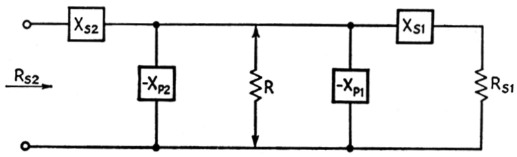
Fig. 10. T network formed from two L sections.
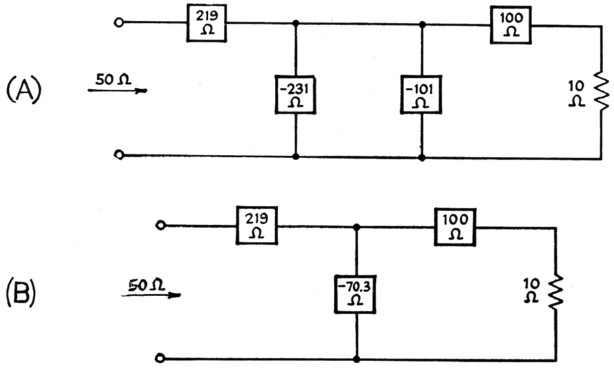
Fig. 11. Combining L-section elements into the T configuration. Note that since the shunt element is formed from two elements in parallel the resultant reactance is less than either alone.
10RS1 = 10 × 10 = 100 ohms. From Equation 2A, R = 10 (102 + 1) = 10 × 101 = 1010 ohm and from Equation 2B,
![]()
The Q required for matching R to RS2 is found from Equation 5:
![]()
so
![]()
and
![]()
The elements of the complete network are shown in Fig. 11, which compares with Fig. 8. The choice of signs is again arbitrary, since the only requirement is that the signs be opposite for the two elements of each L network. In Fig. 11A the parallel or shunt elements have been chosen with the same sign, and so can be combined into a single element, as shown in Fig. 11B.
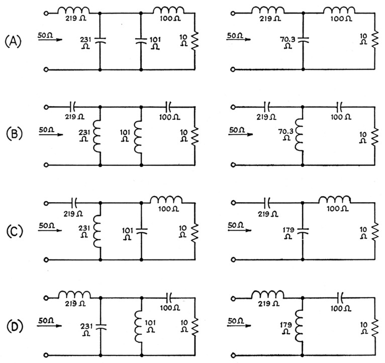
Fig. 12. The four possible combinations of L sections into T networks. The development is shown at the left; final forms at the right.
If different signs are chosen for the reactances, there again result four possible combinations as shown in Fig. 12. As compared with the pi configurations in Fig. 9, the reactances that can be combined are in parallel instead of series, and so the net reactance is not given by simple algebraic addition. However, it is easily found: it is equal to the product of the two reactances divided by their sum, if they are of the same kind (i.e., both capacitive or both inductive); or to the product divided by their difference, if they are of opposite kinds. In the latter case, the net reactance has the same sign as the smaller of the two; in Fig. 12C, for example, the capacitive reactance, 101 ohms, is smaller than the inductive reactance, 231 ohms, and so the net reactance, 179 ohms, is capacitive. The opposite is true in Fig. 12D.
Notes
- For discussion of tank-circuit Q, see chapter on transmitters in The Radio Amateur's Handbook.
- Bruene, "Pi-network calculator", Electronics, May, 1945.
- I particular, the use of the negative sign in this and similar examples should not be confused with the use of the same sign to indicate capacitive reactance. The method of calculation described here does not require such use of signs nor is it necessary to bring the operator j into the calculations.
- Somewhat more complicated formulas must be used for finding the exact values when the series inductance (not reactance) is constant. They are
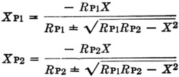
where I is the total reactance of the series inductance, Fig. 9A. For Fig. 9A, use the plus signs in the denominators, in which event the minus signs in the numerators indicate that the shunt reactances are capacitive. In the general case, the same sign must be chosen for both denominators, but X may be either positive or negative. This leads to the four possible combinations shown in Fig. 9. For further details see W. L. Everitt, Communication Engineering, McGraw-Hill Book Co., New York.
Part 1 - Part 2 - Part 3
George Grammer, W1DF.