Simplified design of impedance-matching networks 3
Some Special Applications
The concluding article of this series discusses the problem of loads that can vary over a range of impedances, and describes some useful applications of network principles.
Readers who have followed the discussion in Parts 1 and 2 of this series should have no difficulty in perceiving that the same methods can be used to construct more complicated networks, whenever there is occasion for using something more elaborate than the L, pi and T. The L section is the building block in each case, and a great variety of circuits is possible. A few of the more useful arrangements are discussed below. First, however, it is necessary to say something about matching a range of impedances with a given network, the earlier discussion having been confined to the case where the load is a pure resistance of fixed value. The most important practical case is a pi-network tank circuit connected to a transmission line.
Load-impedance range
The input impedance of a transmission line will be a pure resistance equal to the line's characteristic impedance, Z0, only when the line is perfectly matched at its output end. If there are standing waves on the line the input impedance may be reactive as well as resistive, and the resistance will not, in general, be of the same numerical value as the line Z0.
In this application of the network the design limits for matching will be determined by the range of variation of line input impedance. This in turn is a function of the standing-wave ratio and line length. Considering the line input impedance to be represented by a resistance and reactance in parallel, as in Fig. 13, the extremes of resistance and reactance variation are given by the following table:
| S.W.R. | Min. X | Min. R | Max. R |
|---|---|---|---|
| 2 to 1 | 1.3Z0 | Z0/2 | 2Z0 |
| 3 to 1 | 0.75Z0 | Z0/3 | 3Z0 |
| 4 to 1 | 0.5Z0 | Z0/4 | 4Z0 |
| 5 to 1 | 0.4Z0 | Z0/5 | 5Z0 |
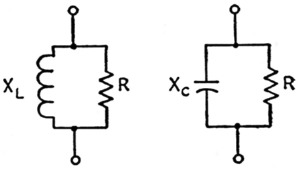
Fig. 13. Parallel-circuit equivalents of transmission-line input impedance.
The reactance figures are rounded, but are close enough for design purposes. (The maximum reactance in this equivalent input circuit will be infinite - meaning, merely, that it can be ignored, since it is in shunt with the resistance.) The worst case, so far as compensating for reactance is concerned, is minimum X. It may be either inductive or capacitive.
The first thing to find, then, is what the maximum s.w.r. will be. This may be a matter of the known characteristics of the antenna system, or an arbitrary limit may be set from other considerations such as line loss. Losses in coax will not be increased intolerably if the s.w.r. is as high as 3 to 1. From the table, the minimum shunt reactance will be 0.75Z0 for this s.w.r., and the load resistance will vary from Z0/3 to 3Z0. In terms of 52 ohm line, for example, this means that the minimum shunt reactance presented to the output terminals of the network by the line will be 0.75 × 52 = 39 ohm, and that the resistance can be anywhere between 17 ohm and 156 ohm. The actual values in a given case will depend on the line length.
The reactance and resistance can be treated separately. If we eliminate the effect of the reactance first, we are then left with a simple resistance load, and this can be handled by the method described in Part 2. Fig. 14 shows the two possible cases. If the reactive component of the line input impedance is capacitive, as at A, it is obvious that X2 and XC are in parallel; that is, the capacitance represented by the reactance XC adds to the capacitance of X2. If the pi network has been designed to match R without considering XC, the presence of XC will destroy the match. However, this is handled quite easily by reducing the capacitance of X2 until the total capacitance, both physically in the output capacitor of the pi network and inherently in the line input impedance, is equal to the proper design value. Provided the capacitance of X2 is continuously adjustable from essentially zero to its maximum value, it will usually be possible to get complete compensation by simple adjustment of the pi-network output capacitance.
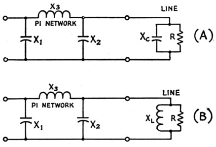
Fig. 14. Equivalent circuits of line input impedance connected to output terminals of a pi-network tank circuit.
If the line input impedance is inductive, as in Fig. 14B, the effect is opposite to that just described - that is, the capacitance of X2 must be increased to compensate. Actually, enough additional capacitance must be supplied to resonate with XL at the operating frequency. This forms a parallel-resonant circuit that, in effect, removes XL from the circuit. The total capacitance required in X2 then is the original design value for matching R plus the additional capacitance needed to resonate with XL.
The minimum capacitive line reactance to be expected with 52 ohm line and an s.w.r. of 3 to 1, 39 ohm, is equivalent to a capacitance of 1170 pF, at 3500 kc. At this frequency, therefore, the actual output capacitance in use in the network will be reduced by 1170 pF from the value theoretically required for matching. On the other hand, if the line input reactance is inductive, 1170 pF will have to be added to the theoretical network output capacitance to compensate. In terms of actual' components, the lower frequencies obviously present the most difficult case because low reactances mean large values of compensating capacitance.
The variation in the resistive component of the line input impedance affects both the series inductance and output shunt capacitance of the network. For a 3-to-1 s.w.r. the load resistance may vary over a 9-to-1 range. The extremes of this range call for quite different network values, particularly if a fairly wide frequency band such as 3500-4000 ke. must be covered. Using the earlier example of a tube requiring a 2000-ohm load, and assuming that the operating Q will be 12 at all frequencies, the inductive reactance values required in the network are 172 ohm for matching 17 ohm, and 210 ohm for matching 156 ohm. The corresponding inductance extremes at 4000 and 3500 kc., respectively, are 6.9 µH and 9.5 µH, so the network inductance should be variable through this range. So far as the output capacitance is concerned, it can be shown that when the virtual resistance R is constant (that is, a constant-Q network) the reactance Xal required for matching in the output L section reaches a minimum value equal to the load resistance when the load resistance is twice the virtual resistance (L-section Q = 1). Since the virtual resistance in the example is 13.8 ohm, the maximum output capacitance will be needed when the load is 27.6 ohm, which also is the value of reactance required. At 3500 kc., this represents a capacitance of 1650 pF.
Fixed tank inductance
When a fixed value of inductance is to he used to cover a band it is necessary to resort to the formulas given in Footnote 9, Part 2, for an exact solution. When the load as well as the frequency are subject to change it is not to be expected that the approximate method described earlier, for a constant load over a frequency band, will work as well, but it will at least serve as a starting point.
In the example above an inductance of 6.9 µH obviously should be chosen, since this is the largest value that will work under all conditions at 4000 kc. and provide the minimum desired Q of 12. At 3500 kc. this inductance will have a reactance of 151 ohm. The assumption that Q will be inversely proportional to frequency requires Q to be 13.7 at 3500 kc. and makes XS1 146 ohm, as shown in Part 2. This is less than 151, but by such a small margin that it immediately suggests that a higher operating Q will be required, especially with load resistances toward the maximum end of the range where XS2 becomes larger. Calculation by the simplified formulas then becomes a matter of trial and error. The actual Q values turn out to be 14.1 when the load is 17 ohm and 16.8 when the load is 156 ohm.
On the whole, it seems desirable to make provision for adjusting the tank inductance values, since this makes for greater flexibility in impedance matching and offers better control over the operating Q. If the inductance cannot be made continuously variable between the limits required for the extreme cases, provision should at least be made for two or more fixed values when attempting to cover a wide band such as 3500-4000 kc.(10) On bands where the width is only a small percentage of the center frequency the problem is of course considerably less difficult. In any case, it is taken for granted that the input and output capacitances will be continuously variable.
The problem of matching a wide range of load impedances over a band of frequencies can be simplified considerably if the network is designed for a fixed value of pure resistance as a load, and then steps are taken externally to make sure that the load presented to the network is the design value. This means that if the actual; load is something else, a special matching circuit is inserted between it and the pi-network tank so the tank sees the load it should. The idea is fundamentally the same as that of using a 115-volt lamp on a 115-volt circuit, instead of trying to make the circuit handle all lamp ratings from, say, 32 volt to 230 volt. In other words, you don't have to rebuild the transmitter when you try out a new antenna system.
The Pi-L
Adding an L section to a pi-network tank circuit increases the flexibility of the system in handling loads varying over a range of impedances and also adds to the selectivity. This combination has been used in commercially built transmitters (e.g., the Collins 32V series) and has the fundamental form shown in Fig. 15A. It may be broken down into three L networks, two of which constitute the pi network as shown in Fig. 7, Part 2 (the same notation for components is used here).
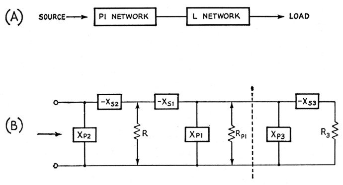
Fig. 15. The pi-L network. The block diagram at B shows the circuit broken down into its L-section components.
The third L is to the right of the dashed line in Fig. 15B; as shown here it is a step-down network looking toward the load, R3, but a step-up network could be substituted if desired. Each of the three L sections would be designed according to the principles previously outlined, keeping in mind the relationships that must be satisfied between the values of the various resistances, real or virtual.
In Fig. 15B there are two virtual resistances, R and RP1, the actual load resistance being R3. Suppose that R3 is 52 ohm, and that the whole network is to be used under the same conditions as the example considered in Part 2 - i.e., to present a 2000 ohm load to the final amplifier tube. In this case a desirable value of tank Q no doubt would be a determining factor, so let us assume that the design value of Q again will be 12. As described earlier, this immediately sets the value of the virtual resistance R, hence XS2 and XP2 also would have the same values as in the previous example: R = 13.8 ohm, XS2 = 166 ohm, and XP2 = 167 ohm.
The network between R and R3 is obviously a T with a virtual resistance RP1. It was shown in Part 2 that this resistance must be higher than either of the resistances, R and R3, being matched. R3, 52 ohm, is higher than R, so RP1 must be larger than 52 ohm if a match is to be possible. Any value larger than this may be selected. If selectivity is the important consideration, a moderately high value of Q will be desirable in one or both of the L sections formed by XS1XP1 and XS3XP3. We may arbitrarily select a Q (Q1) of 5 for the XS2XT2 network. Then XS1 = 5 × 13.8 = 69ohm from Equation 3B, and from. Equation 2A RP1 = 13.8 (25 + 1) = 359 ohm.
Then from Equation 2B
![]()
Thus 52 ohms (R3) must be matched to 359 ohms (RP1) through XS3 and XP3. Following the same method, the Q (Q3) of this network is (Equation 5)
![]()
Hence from Equation 2B
![]()
and from Equation 3B
![]()
Broken down into these components, the complete network is shown in Fig. 16A, where the reactance signs again mean nothing more than that opposite kinds of reactance must be used in each L network. The various physical circuit combinations that are possible can be appreciated by visualizing the output L section in either of its two forms - series inductance and shunt capacitance, or series capacitance and shunt inductance - combined with each of the four forms of the pi network shown in Fig. 9, Part 2. However, since it was assumed that the L section was being added primarily for additional selectivity, particularly against harmonics of the operating frequency, the probability is that it will consist of shunt capacitance and series inductance. Added to the pi network using similar shunt and series arms, the final appearance of the network would be as in Fig. 16C.
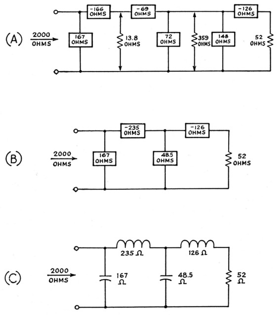
Fig. 16. Pi-L network example discussed in the text.
In Part 2 it was stated that if the tank inductance - that is, the series arm - of the pi network has a fixed value for a given band, matching can only be effected between two given values of resistance by varying the operating Q of the network. If the output inductance of the pi-L is adjustable, the operating Q can be held constant throughout a band even though the pi-section inductance is fixed. This is because the virtual resistance RP1, Fig. 15B, may be varied at will, so long as it is larger than either R or R3. Thus in Fig. 16 the pi-section inductive reactance of 235 ohm will represent an inductance of 10.7 µH at 3500 kc. At 4000 kc. the same inductance will have a reactance of 268 ohm. Of this, 166 ohm will represent the series inductance of the input L of the pi section, for constant operating Q, so the remainder, 102 ohm, is the series inductance XS1 of the output L of the pi section. This leads to a new value 102 / 13.8 = 7.4 as the Q (Q1) of this L section and a corresponding value of 770 ohm for the virtual resistance RP1, instead of the 359 ohm shown in Fig. 14. The new values of XP1, XP3, and XS3 may readily be calculated from this.
Note that a variable inductance is still required for working over a range, just as in the case of the plain pi network discussed above (this example considers only a frequency range, but similar considerations apply where the load can vary). In the pi-L the variable-inductance element merely may be transferred out of the pi. This is exactly the same thing as the "external" network suggested in the discussion of matching a range of impedances with the pi.
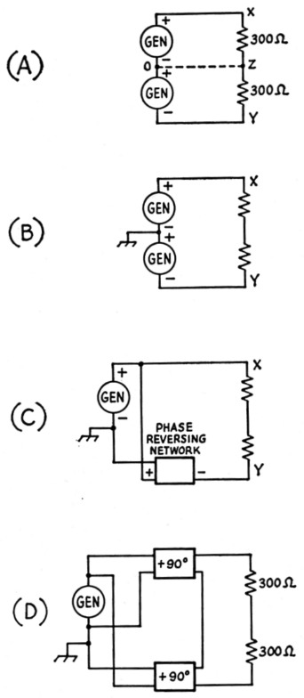
Fig. 17. Development of the balun network.
Balun networks
A common problem is that of matching a balanced or push-pull load to an unbalanced or single-ended source of power. A balanced load, in usual nomenclature, is one having its outside ends equally "hot" (but in opposite phase) with respect to a center point which in the ordinary case may be grounded. We may consider such a load, assuming it to be resistive only, as consisting of two identical resistances in series, each having a value of one-half the total resistance.
Thus Fig. 17A shows a 600 ohm load divided into two 300 ohm sections connected together at Z. If the load is supplied from two d.c. generators each delivering, say, 100 volt, then the potentials at points X and Y will both differ from that at Z by 100 volt. With the polarities as shown, X will be positive and Y will be negative with respect to Z. As viewed from Z, this is equivalent to saying that the voltages at X and Y are 180 degrees out of phase, although they are acting in series around the circuit as a whole.
Since the two generator voltages are equal and so are the two resistances, points Z and 0 are at the same potential. Hence a connection as indicated by the dashed line may be made without disturbing the operation of the circuit.
With this as background, imagine the two 300-ohm resistors in Fig. 17 to represent the input impedance of a matched transmission line. Z is a "neutral" point, and may be taken to be at ground potential if the line itself is reasonably well balanced to ground. When this is so two equal-voltage generators, each having one terminal grounded, can be used to supply power to the line, provided their voltages are out of phase when viewed from the ground point (Fig. 17B). As an extension of this idea, both sides of the line could be fed from a single generator by connecting one side directly to the generator and feeding the other through some sort of network, such as a transformer, that would reverse the phase or polarity without changing the voltage. This arrangement, shown in Fig. 17C, has a fixed 4-to-1 impedance ratio since the voltage that is applied to the load cannot be other than twice the generator voltage.
For maximum flexibility the arrangement shown at Fig. 17D can be used. There are two networks in this circuit, one for each side of the line. Each provides a 90-degree phase shift, but in opposite directions, so that the total is the necessary 180 degrees. In addition, each network can be designed to give a voltage step-up or step-down - i.e., to match any desired impedance values - along with the proper phase shift. The same impedance ratio must be used in both networks, of course, since the load is balanced. The pi network lends itself nicely to this application.
The question of phase shift through a network has not been considered up to this point, since it is unimportant in the types of applications discussed earlier. It does not in fact require any extended discussion here, even though it is important in the balun, because the case of interest - the one where a plus or minus shift of 90 degrees is obtained - is a quite simple one. In the pi network a phase shift of 90 degrees results when the maximum value of reactance that will provide a match between two resistances is used in the series arm. This value of reactance is equal to the geometric mean of the two resistances to be matched - that is,
![]()
where R1 and R2 are the two resistances. In this case also the shunt arms XP1 and XP2 have equal reactances of the same absolute value as XS, but of course of the opposite type. There will be a lagging phase shift through a pi network having series inductance and shunt capacitance, and a leading phase shift through one with series capacitance and shunt inductance.
Suppose that the 600 ohm balanced line is to be matched to a 52 ohm coaxial line. Using the basic arrangement of Fig. 17D, there will be two networks, operating in series insofar as feeding the balanced line is concerned. Each network therefore will see a 300 ohm load. On the input side the generator must see a 52 ohm load. What it actually sees is the two networks connected in parallel, so each network must have an input resistance of 104 ohm. Thus each network must be designed to match 300 ohm to 104 ohm.
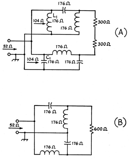
Fig. 18. A - Circuit elements in the balen.
B - Actual circuit after eliminating the parallel-resonant circuit formed by L1 and C1.
The circuit configuration that this leads to is shown in Fig. 18A. The reactances required in each network for a match are
![]()
Note that L1 and C1 are in parallel, and since they have the same reactances they form a parallel-resonant circuit. Such a circuit has infinite impedance (this is not strictly true if there are any losses in the coil and capacitor, but in actual applications of this circuit it is practically so if the circuit elements are reasonably low-loss) and this being the case, these two components can be lifted out of the circuit without change in its operation. This leaves the relatively simple configuration shown in Fig. 18B.
Pi networks using this design have the minimum possible operating Q (the actual value of Q will vary with the ratio of the resistances to be matched) and so have maximum band width. A balun circuit having fixed values of inductance and capacitance will work well over an entire amateur band if it is designed for the band center and if the actual load (transmission line input impedance) remains resistive and constant over the entire band. It is unfortunate that a practical transmission-line load is seldom that accommodating.
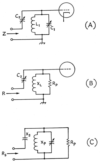
Fig. 19. Reactance adjustment making use of the properties of a tunable circuit of parallel inductance and capacitance near resonance.
Not-so-obvious forms
A few fairly familiar coupling circuits have the interesting characteristic of appearing to be one thing and actually operating like something else. An example is the antenna input circuit on some military receivers such as the BC-348 series where a small variable capacitor was used for coupling adjustment between a low-impedance line and the grid circuit of the first r.f. tube. This looks like a rather makeshift method that could not possibly come close to giving maximum power transfer. Actually it is a form of L network and is capable of providing a quite good match.
The essentials of the circuit are shown in Fig. 19A. L1C1 is a circuit capable of being tuned to and around the operating frequency, while C2 is a variable capacitor having a relatively small maximum capacitance. When L1C1 is tuned exactly to the operating frequency it will have a purely resistive impedance of some tens of thousands of ohm, if the circuit losses are low. The impedance Z, looking into the input terminals, is simply the combination of this resistance and the reactance of C2 in series.
However, if L1C1 is not tuned to resonance but is tuned off on the low-frequency side, its impedance can be represented by a resistance and inductive reactance in parallel, as shown in Fig. 19B. This will be recognized as an L network, and the matching possibilities should immediately be apparent. The inductive reactance, XL, and equivalent parallel resistance, Bp, of the circuit are both varied by adjustment of C1. The reactance of C2, also adjustable, is the series arm of the L network, and so proper adjustment of both C1 and C2 will bring about an impedance match between the "tuned" circuit and a low-impedance line. Thus maximum power will be taken from the line when L1C1 is not tuned to resonance.
The device of using a parallel LC circuit to obtain smooth variation of inductive reactance can be and has been used in transmitting circuits. In Fig. 19C the LC combination is merely an adjustable Xp, using the notation of Part I for the L network. Xs would be computed in the usual way. For Xp it is only necessary to provide a parallel circuit capable of being tuned through resonance at the operating frequency. Since there will be circulating current in this circuit and consequent higher internal loss than if a simple inductance of the proper value were used, it is advantageous to use a high-Q coil and a high L/C ratio. However, the efficiency is always less than with the simple inductance, if equally good coils are used in both cases.
Conclusion
The design methods that have been described are essentially simple and, once the physical principles by which impedance transformation takes place are thoroughly understood, can be applied without recourse to books or other references if the one basic relationship is kept in mind: The equivalent parallel resistance of a circuit containing resistance and reactance in series is equal to the series resistance multiplied by (Q2 + 1). Everything follows from that, by elementary algebraic manipulation. You have to know the definitions of Q and reactance, of course, but these are prerequisites for anyone who hopes to undertake the design of coupling circuits - or the design of radio circuits of any type, for that matter.
notes
- The writer has used a small tapped auxiliary coil for providing relatively fine adjustment of inductance, with a separate switch, where a large number of taps on the main tank inductance was inconvenient.
Part 1 - Part 2 - Part 3
George Grammer, W1DF.