Array design with optimum antenna spacing
Getting the most gain from stacked antennas.
Stacking two antennas doesn't always result in a 3 dB, gain improvement - it all depends on the spacing used. Here's down-to-earth information on putting together multi-antenna arrays complete with universal design charts and examples of how to use them.
In the April, 1958 issue of QST, the author presented an article entitled "Optimum stacking spacings in antenna arrays." It soon became evident that although basic terms and fundamental equations were used in an effort to attain simplicity, many people did not grasp the meaning of the concepts presented nor were they able to utilize these concepts in a practical antenna design. The following words of wisdom were assembled to assist these people.
The first part of this article is a brief review of the original material, while the second part presents practical antenna designs fashioned in response to various inquiries.
Need for optimum spacings
Many amateurs, especially v.h.f. enthusiasts, have become aware that an antenna, no matter how small it is physically, has associated with it a power-gathering area. This area is called " effective aperture," and more often "capture area."
As an example, consider the dipole. The maximum effective aperture of a dipole is approximately the same as an area ½ by ¼ wavelength on a side. The physical significance of this aperture is that the power from the incident plane wave is absorbed over an area of this size by the dipole, and is delivered to its terminating resistance.
With the increasing use of multielement Yagis, it became evident that longer Yagis had larger "effective apertures," and that in order to realize maximum gain when using two stacked Yagis, a spacing larger than the customary half wavelength was needed to insure that the respective capture areas were not "overlapping." The same effect was noted in the case of collinear dipoles, where a center-to-center spacing of approximately ¾ wavelength is needed to achieve maximum gain. It should be noted that the customary half-wavelength spacing is a carry-over from collinear array design where no side lobes are desired. For an amateur striving to achieve maximum gain, an antenna design utilizing half-wavelength spacings between elements can be termed inefficient!
Achieving optimum spacings
The presence of a capture area poses two important questions:
- How does the capture area vary with different antennas?
- In stacking antennas, how must the individual capture areas to be positioned for maximum efficiency?
The first question can be answered intuitively. The higher the antenna gain, the larger is the capture area.
The answer to the second question cannot be obtained so easily. Although the capture area can be expressed mathematically, its exact geometrical configuration remains unknown. Fortunately, there is a method which enables us to compute the spacings necessary for achieving maximum gain. This method utilizes an important principle of antenna design called "pattern multiplication." It is restated here for the personal edification of those not in the know: "The field pattern (note: field, not power) of an array of nonisotropic but similar point sources (i.e., an array of dipoles, or Yagis, or horn antennas, etc.) is the product of the pattern of an individual source and the pattern of an array of isotropic point sources, having the same locations, relative amplitudes and phases as the nonisotropic sources." A thorough explanation of this statement, plus array patterns for isotropic point sources, can be found in Antennas, by Kraus.
Now suppose we have several Yagis and wish to stack them. How do we calculate the proper spacing for maximum gain? The necessary steps are as follows:
- Determine the field pattern of an individual Yagi (i.e., rotate it and plot the field strength).
- Determine the proper array factors or patterns for various spacings from Antennas.
- Multiply the two to obtain the field pattern of the array.
- Calculate the gain for the various spacings from the beam widths (see author's article in April, 1958, QST).
- Calculate the level of the highest side lobe for the various spacings. (Maximum gain occurs at approximately a -13 dB [0.22 in voltage] side-lobe level.)
Lots of work? You bet it is. The plots and calculations become quite cumbersome, especially when the number of antennas to be stacked becomes large. In order to simplify things, the author assumed "typical" field patterns for antennas having various beam widths. Following the procedure outlined above, a plot of optimum stacking spacing vs. antenna beam width was obtained. The results are shown here in Figs. 1 and 2. Figs. 3 and 4 were given by Greenblum(1) in a previous article and illustrate the beam widths obtained from multielement Yagis. By using these charts, we can quickly determine the optimum spacing for a given array design.
Figs. 1 and 2 are similar to the curves shown in the author's previous article, but close examination will show a difference, especially in the maximum gain curves. The reason for the change is as follows: Originally a 10 dB side-lobe level was taken as the point at which maximum gain occurs. However, a little thought on the subject led to the conclusion that a 13 dB side-lobe level would be more appropriate. As shown by Silver,(2) a uniformly illuminated rectangular aperture exhibits maximum gain at a side-lobe level of -13 dB, while for a uniformly illuminated circular aperture maximum gain occurs at a side-lobe level of -17.6 dB. It can be seen that stacking several antennas will result in an approximate uniformly illuminated rectangular aperture. The approximation is even more exact when a large number of antennas is stacked.
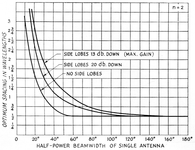
Fig. 1. Optimum stacking spacing for two antennas (n = 2). The spacing for no side lobes can result in little gain over a single source, especially with small beam widths.
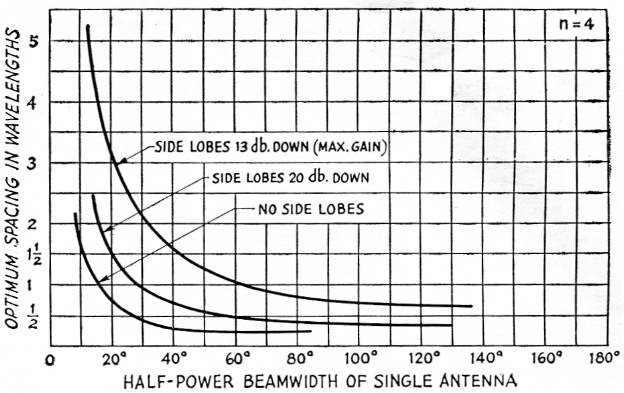
Fig. 2. Optimum stacking space for four antennas (n = 4). Note: Spacings less than'/ wavelength are physically possible only for shortened dipoles in the case of collinear elements or for stacking in the plane perpendicular to the plane of polarization.
Practical designs
Stacking quad antennas
During recent years, the "cubical quad" or "bi-square" antenna has been enjoying increasing popularity. Here is a typical problem posed to the author by John Knight, W6YY, concerning the stacking of two quads. The quads are to be stacked horizontally and will replace a three-element Yagi.
The following questions were raised:
- Can one consider the cubical quad when stacked horizontally to behave the same as collinear dipoles in phase for the graphs and calculations given?
- What is the "best" horizontal spacing, center-to-center, for two quads to produce the best forward gain and directivity with optimum side lobes?
The answer to the first question is affirmative. The optimum spacing curves are universal; i.e., they can be applied to the quad, loop, slot, dipole, or any type of antenna. This is because the calculations were based on beam width, and not on any particular antenna type. The only restriction imposed is that the individual patterns have no side lobes. Actually, the results will hold for patterns with moderate side-lobe levels, since the multiplication process reduces their level.
To answer the second question, let us first determine the spacing for -13 and -20 dB side-lobe levels and then outline the steps leading to a final selection. In order to find out the spacing values we must know the horizontal beam width. Assuming that the horizontal and vertical beam widths are approximately equal, their value can be calculated from the expression
Gain (db.) over isotropic source
![]()
where θh and θv are the horizontal and vertical beam widths in degrees. A dipole has 2.14 dB gain over an isotropic source (one that radiates energy uniformly in all directions), so a quad with 6 dB gain over a dipole will have 8.14 dB gain over an isotropic radiator. Therefore,
![]()
and θh = 80°.
From Fig. 1 we see that for an 80-degree beam width a spacing of 0.73 wavelength is appropriate for a -13 dB side-lobe level, while 0.64 wavelength spacing would reduce the side-lobe level to -20 dB. The difference in gain for the two spacings would be about 1 dB and this would be hard to detect with most measurement techniques. The final spacing choice is one of personal preference. However, the following points can be used as guides in making the choice:
- Lower side-lobe levels reduce interference when the band is highly populated.
- Smaller spacings require less boom length and are desirable from a mechanical viewpoint.
- In some cases a large spacing will create physical problems in impedance matching.
The 8 over 8 for 2 meter
The 8-element Yagi has become a popular 2-meter antenna. In order to stack two, we proceed as follows: Fig. 3 shows that an 8 element Yagi has a beam width of approximately 37 degrees in the plane of polarization (i.e., horizontal plane for a horizontal Yagi). The vertical beam width is slightly larger, but for all practical purposes the two can be considered equal. For two Yagis (n = 2) we see from Fig. 1 that a stacking spaceing of 1M wavelengths is needed in either plane for optimum performance. Using a design frequence of 145 Mc. (free-space wavelength = 81.4 inch) the 1½ wavelength spacing is 10 feet, 2 inch. Deviations from this spacing of a few inches can be tolerated without any noticeable degradation of performance.
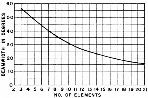
Fig. 3. "E"-plane half power beam width of a Yagi vs. number of elements (including one driven element and one reflector). The "E" plane is the plane of polarization of the signal; in this case it corresponds to the plane of the antenna elements.
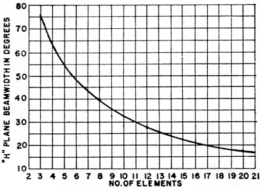
Fig. 4. "H"-plane half power beam width of a Yagi vs. number of elements (including one driven element and on reflector). The "H" plane is the plane at right angles to the plane of polarization.
Fig. 5 shows two configurations for feeding the Yagis, assuming each Yagi has a feed point impedance of 450 ohms. The spacing in Fig. 5A is optimum, while that in Fig. 5B is a few inches less to facilitate impedance matching. In Fig. 5A an open-wire line of any characteristic impedance connects the two Yagis. Each half of this line is electrically one wavelength long. Using a velocity factor of 0.975 this comes out 79.4 inches. The impedance at the midpoint is half that of each beam or 225 ohm. A 4-to-1 impedance transforming balun connected at this point transforms the 225 ohm to 56 ohm and also provides the change from balanced to unbalanced line. If a balanced transmission line is desired, 300 ohm Twin-Lead can be used between the midpoint and the balun.
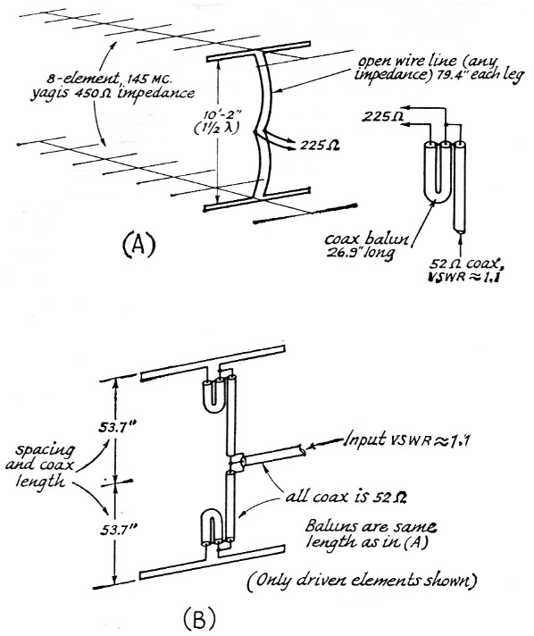
Fig. 5. (A) Two 8-element Yagis for 145 Mc. stacked with optimum spacing of 1½ wavelengths. The open-wire line connecting the antennas is 2 electrical wavelengths long (with a velocity factor of 0.975). The balun and 52 ohm coax can be mounted right at the 225 ohm midpoint, or a 300 ohm transmission line can be used between them.
(B) Alternate matching system using only coax. The spacing between Yagis has been reduced slightly to accommodate the 2-wavelength coaxial phasing line (velocity factor 0.66).
Fig. 5B shows a similar scheme which will provide equal performance and uses all coax rather than an open-wire line phasing section. In this method two baluns are used, one being placed directly at the feed point of each Yagi. The 450 ohm balanced is transformed to 112 ohm unbalanced, and the two baluns are then connected through a piece of coaxial line having a half length of 53.7 inch. Again this half length is electrically a wavelength long (using a velocity factor of 0.66). At the midpoint of the coax line the impedance is 56 ohms, and at this point a direct connection can be made to standard RG-8/U or RG-58/U coaxial cable.
The open-wire line used in Fig. 5A minimizes feeder and balun losses. However, actual measured balun losses using RG-8/U ran less than 0.1 dB at 145 Mc, and the use of coax minimizes the chance of feeder radiation.
A stacked array for satellite reception
Fig. 6 shows two vertical 5-element Yagis stacked horizontally for maximum gain. The lengths and spacings given are for 108 Mc. The beam width of one antenna in the plane perpendicular to the plane of polarization as given by Fig. 4 is 54 degrees. The stacking spacing for maximum gain with two such antennas (n = 2) can be taken from Fig. 1 as 13 wavelengths. Notice that we are only concerned here with picking up the satellite signals and not with any phase-comparison system such as Minitrack, which has special spacing requirements.
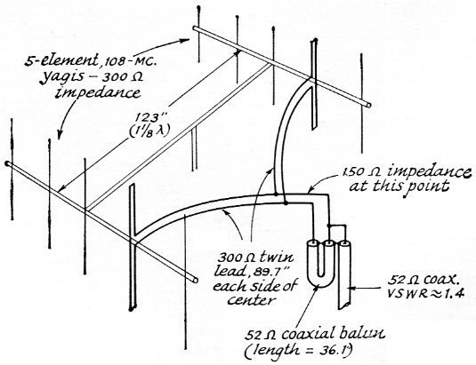
Fig. 6. Matching system for two 5-element Yagis with optimum spacing of 1_1/8 wavelength. Dimensions are for 108 Mc. The Twin-Lead connecting the two antennas is 2 wavelengths long with a velocity factor of 0.82.
Each Yagi is connected to a piece of 300 ohm Twin-Lead one wavelength (89.7 inches using a velocity factor of 0.82) long. The two lengths of Twin-Lead are tied in parallel, resulting in a midpoint impedance of 150 ohms if the Yagi feed-point impedances are 300 ohms. A 4-to-1 balun connected to the midpoint will transform this to about 38 ohm unbalanced and can be fed directly with RG-8/U or RG-58/U cable.
Notes
- Greenblum, "Notes on the development of Yagi arrays," Part 1, QST, August, 1956.
- Silver, "Microwave antenna theory and design, MIT Rad. Lab. Series, Vol. 12.
H.W. Kasper, K2GAL.