Key components of modern receiver design 1
Today's Amateur Radio receivers routinely achieve performance untouched by earlier generations of ham gear. Can our already excellent equipment be improved still further?
The fact that many presentations have dealt with receiver capabilities and improvements over the years might seem to imply that all receiving problems have been solved and that the technology is mature. On the other hand, a look at the components actually used in the front ends of current receivers by different manufacturers indicates that just the opposite is true. While improvements have been made in mixers, amplifiers and synthesizers-and from a systems point of view there have been some subtle implementations of individual circuits-there is still work to be done! How else can one explain that different receiver designs-with similar block diagrams, and brought to market with the best of intentions-sound different on the air?
Modern ham equipment seeks to achieve high dynamic range in relatively standard, seemingly well-established ways. Nonetheless, I have discovered that it's useful to reevaluate the definition of dynamic range, and how AGC and gain distributiop affect it. As part of this discussion, I will show how to overcome the effects of a form of intermodulation distortion long thought unimportant in ham circles-a species of RF IMD that noticeably degrades reception even in high-end Amateur Radio MF/HF transceivers.
Likewise, we may benefit by revisiting the influence of oscillator phase noise on dynamic range, and the well-known interdependence of fast PLL settling time and phase noise. After discussing my findings, I will propose a hybrid synthesizer arrangement-a DDS-driven PLL system-and show how commercial CAD can now accurately predict the SSB phase noise of oscillators and provide the ability to optimize it.
Dynamic range types and issues
There are several types of dynamic range. The first one, and probably the easiest to understand-"AGC range"-concerns whether a receiver is capable of maintaining a constant audio output level over a large input-signal amplitude range. The traditional school of thought requires AGC action to commence at 1 or 2 µV, leading to a condition where signals that produce an excellent signal-to-noise ratio may show absolutely no S-meter indication-a most undesirable effect. The reason for this is inappropriate receiver gain distribution-generally, a lack of gain at the second IF. Maintaining constant audio output must involve gain control at the receiver's second and first IFs, and possibly even at its input. I will address this issue later.
Intermodulation-distortion dynamic range
The output of a linear stage tracks the input signal decibel by decibel, with every 1-dB change in its input signal(s) corresponding to an identical 1-dB output change. This is the stage's first-order response.
Because no device is perfectly linear, however, two or more signals applied to it intermodulate to some degree, generating sum and difference frequencies. These intermodulation distortion (IMD) products occur at frequencies and amplitudes that depend on the order of the IMD response as follows:
- Second-order IMD products change 2 dB for every decibel of input-signal change,(1) and appear at frequencies that result from the simple addition and subtraction of input-signal frequencies. For example, assuming that its input bandwidth is sufficient to pass them, an amplifier subjected to signals at 6 and 8 MHz will produce second-order IMD products at 2 MHz (8 - 6) and 14 MHz (8 + 6).
- Third-order IMD products change 3 dB for every decibel of input-signal change,(2) and appear at frequencies corresponding to the sums and differences of twice one signal's frequency plus or minus the frequency of another. Assuming that its input bandwidth is sufficient to pass them, an amplifier subjected to signals at 14.02 MHz (f1) and 14.04 MHz (f2) produces third-order IMD products at 14.00 (2f1 - f2), 14.06 (2f2 - f1), 42.08 (2f1 + f2) and 42.10 (2f2 + f1) MHz. The subtractive products (the 14.00 and 14.06-MHz products in this example) are close to the desired signal and can cause significant interference. This is why our receivers' third-order IMD performance is so important.
It can be seen that the IMD order determines how rapidly IMD products change level per unit change of input level. Nth-order IMD products therefore change by n dB for every decibel of input-level change.
IMD products at orders higher than three can and do occur in communication systems, but the second- and third-order products are most important in receiver front ends.
Intercept point
The second type of dynamic range concerns the receiver's intercept point, sometimes simply referred to as intercept. Intercept point is typically measured by applying two or three signals to the antenna input, tuning the receiver to count the number of resulting spurious responses, and measuring their level relative to the input signal.
Because a device's IMD products increase more rapidly than its desired output as the input level rises, it might seem that steadily increasing the level of multiple signals applied to an amplifier would eventually result in equal desired-signal and IMD levels at the amplifier output. Real devices are incapable of doing this, however. At some point, every device overloads, and changes in its output level no longer equally track changes at its input. The device is then said to be operating in compression. Pushing the process to its limit ultimately leads to saturation, at which point input-signal increases no longer increase the output level.
The power level at which a device's second-order IMD products equal its first-order output (a point that must be extrapolated because the device is in compression by this point) is its second-order intercept point. Likewise, its third-order intercept point is the power level at which third-order responses equal the desired signal. Figure 1 graphs these relationships.
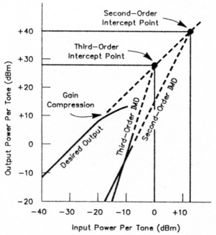
Figure 1-A linear stage's output tracks its input decibel by decibel on a 1:1 slope-its first-order response. Second-order intermodulation distortion (IMD) products produced by two equal-level input signals ("tones") rise on a 2:1 slope-2 dB for every 1 dB of input increase. Third-order IMD products likewise increase 3 dB for every 1 dB of increase in two equal tones. For each IMD order n, there is a corresponding intercept point IPn at which the stage's first-order and nth order products are equal in amplitude. The firstorder output of real amplifiers and mixers falls off (the device overloads and goes into compression) before IMD products can intercept it, but intercept point is nonetheless a useful, valid concept for comparing radio system performance. The higher an amplifier or mixer's intercept point, the stronger the input signals it can handle without overloading. The input and output powers shown are for purposes of example; every receiver exhibits its own particular IMD profile. (After W. Hayward, Introduction to Radio Frequency Design, Figure 6.17)
Input filtering can improve second-order intercept point; device nonlinearities determine the third, fifth and higher-oddnumber intercept points. In preamplifiers, third-order intercept point is directly related to dc input power; in mixers, to the local-oscillator power applied.
Intercept point can be confusing because it can be specified in terms of input or output power. Intercept point should be referred to device output because that's where the trouble occurs, but input intercept is commonly given. Therefore, if an amplifier or a mixer has a particular intercept point-let's say +30 dBm at 10 dB gain-and then its gain is increased by an additional 10 dB, its dynamic range decreases by the amount of the gain.
A good example of this confusion is the highly acclaimed Plessey SL6440C active mixer. DeMaw and Collins(3) evaluated this device with 200-Ω input and output terminations. Their findings were based on a device gain of 8 dB, maximum, and an output intercept point of +30 dBm. By the time the SL6440C's output impedance is raised to 1.5 kΩ on each collector, all other things being equal, its intercept point deteriorates to about +10 dBm. The additional gain favors the intermod products, degrading the intercept point by 20 dBm and destroying the mixer's dynamic range. It's therefore highly desirable to keep mixing and amplification functions separate-mixer first, amplifier second. A smart way to accomplish this is to put a crystal filter between the two to band-limit the spectrum, and thus the signal power, applied to the postamplifier. More on this concept later.
Blocking and desensitization
Because of its noise sidebands, a receiver's synthesizer mixes adjacent-channel signals into the IF chain as noise even though the signals themselves fall outside the IF passband. The result is a degradation of receiver noise floor known as blocking or desensitization.(4)
In addition, synthesizers are frequently dirty-spectrally impure-specifically if complicated mix and divide arrangements are used. Even most modern direct digital synthesizers do not take advantage of configurations that minimize unwanted spurious response. In this article, I will look at a way of drastically improving a synthesizer's output purity while reducing costs at the same time.
Tone spacing and measurement results
Dynamic-range characteristics that involve two or more signals also depend on the signals' frequency spacing. In the standard case, where the desired, low-level signal is bothered by a stronger signal, a receiver's performance drastically varies as a function of the spacing between the two. Most receiver measurements of this type are conveniently done at a test-signal ("tone") spacing of 20 to 25 kHz. Real life is often not so generous! Strong signals may be spaced only a few kilohertz apart, and the receiver's first-IF ("roofing") crystal filter (say, 15 kHz wide) does not protect the second mixer as a much narrower filter, like the 2 to 4-kHz units commonly used for SSB, would do. In a radio using a 15-kHz first-IF filter and a 2.5-kHz second-IF filter, the second mixer must therefore digest the signal energy in 12.5 kHz of spectrum invisible to circuitry after the second-IF filter. The wider roofing filters (Figure 2) used in some amateur equipment makes .life. even harder for the second mixer.
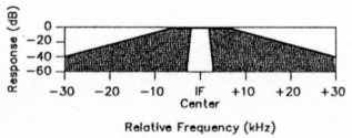
Figure 2-Signals that fall within the passband of a receiver's roofing filter (shaded and unshaded zones under curve) but outside the passband of subsequent narrower filters (unshaded zone) can overload the circuitry between them.
The standard AGC approach derives its control voltage from second-IF energy and does not even acknowledge the existence of these signals. The current trend to replace IF stages with digital signal processing will aggravate this situation even more because A-to-D converters do not respond gracefully to signals that exceed their dynamic range. AGC attack time can therefore be particularly critical in DSPequipped receiving systems even if the AGC range is otherwise adequate.
How to deal with these issues
What do we find
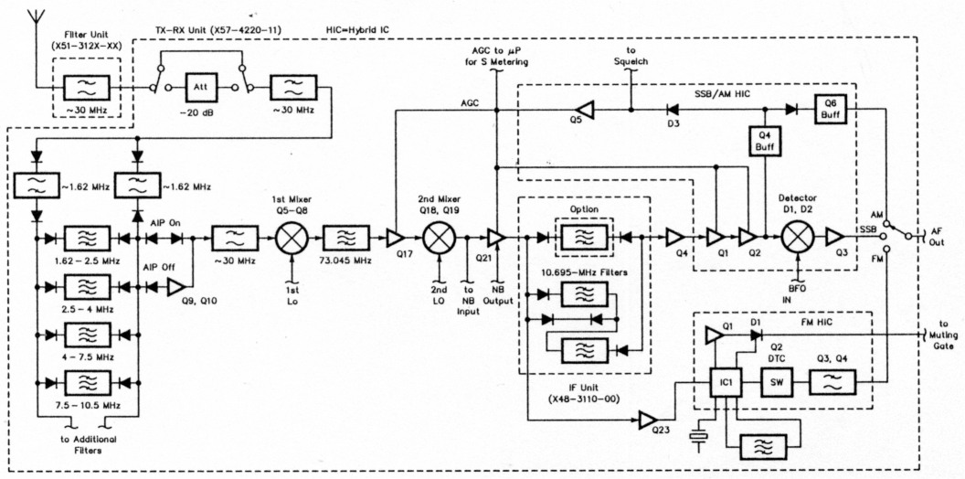
Figure 3-In keeping with general practice in Amateur Radio transceivers, Kenwood's TS-50 applies only second-IF AGC to amplifier stages between its roofing and second-IF filters.
Is the receiver's AGC, selectivity and gain distribution proper? Figure 3 shows the front-end and IF block diagram of a reasonably standard transceiver design-that of the recently introduced Kenwood TS-50 transceiver. The first IF stage of its receiver (TX-RX Unit Q17, a 3SK121 MOSFET) receives AGC, but that this AGC is derived from the output of the radio's second-IF chain. For the reasons described earlier, this system cannot protect the TS-50's second mixer from overload caused by signals inside the roofing filter passband and outside the passbands of the switchable filters that head its second IF. A further drawback of this AGC method is that Q17's third-order intercept point worsens as its gain is reduced-a characteristic intrinsic to MOSFETs that are gain-controlled in this way. Using a differential amplifier or PIN-diode attenuator as the gain-controlled stage would avoid this.
Radios constructed along similar lines often suffer from:
- Insufficient AGC range. Listen to a full-carrier, double-sideband AM signal, modulated at least 50%, at a level of 100 mV or more. You will likely hear distortion because many receivers' AGC circuitry run out of control range by the time incoming signals reach this level.
- Overload related to insufficient AGC if a 20-mV signal that appears 5 kHz away from a properly tuned-in CW or SSB signal falls inside, the roofing filter passband and outside the second-IF filter.
- Desensitization caused by LO spurious signals and phase noise, which can allow strong nearby carriers to raise the receiver noise floor. Does your all-band transceiver allow you to tune to an input frequency of 5 or 10 kHz instead of 500 kHz or higher? Interesting time and standard-frequency signals can be received below 50 kHz, but designers of receivers and transceivers usually disallow tuning below 100 kHz because of their limited synthesizer purity. Your radio's firmware-set lower tuning limit directly reflects how "good" its synthesizer really is.
The right approach
Distributed AGC
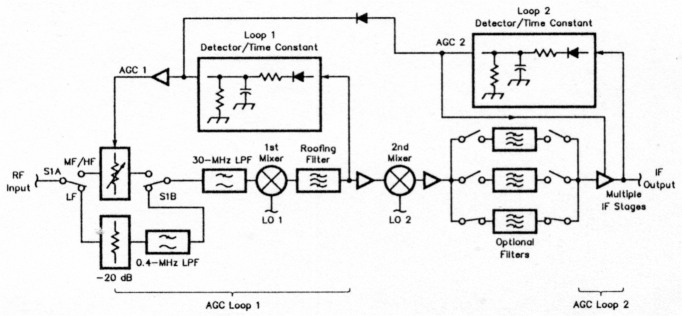
Figure 4-This receiver block diagram includes two AGC loops-one driven by first-IF energy that is band-limited by the roofing filter, and another driven by second-IF energy band-limited by the optional second-IF filters. The first loop controls a PIN-diode pi attenuator ahead of the first mixer; the second loop controls second-IF amplifier stages. A microprdcessor adjusts the time constants of both loops so that time delays introduced by the filters do not cause AGC oscillation. For clarity, this block diagram omits the input filtering (to the left of RF Input) necessary for a practical system.
Figure 4 shows a partial block diagram of a receiver with distributed AGC that includes second-mixer overload monitoring. One AGC loop operates at the front end and protects the input stage with an electronically controlled attenuator. In most radios, this attenuator is manually operated from the front panel and offers a gain-reduction range of perhaps 30 dB in 5, 6 or 10-dB steps. Many operators find its use somewhat confusing because it changes the S-meter indication. Modern microprocessor-controlled radios should be capable of selecting the proper attenuation level and correcting the signal-meter indication appropriately.
Signal-strength metering
S-meter calibration, indication and use have long been somewhat emotional issues in Amateur Radio. I strongly recommend that we redesign our signal meters along the lines of those used by our professional colleagues, calibrating them from -20 dBµV (0.1µV in 50 Ω) to +100 dBµV (100 mV in 50 Ω) - a 120-dB range. Such a system requires that a receiver's AGC system have enough pre-detector gain so that the AGC operates on IF noise alone. Note that, per Table 1, -20 dBµV is close to the extrapolated definition for S0 of about 0.07 µV.(5)
Aside from its objectivity, this arrangement offers the advantage of allowing true comparisons between signals, and accurate system-parameter measurements (such as antenna front-to-back ratio, useful characterization of which is all but impossible with most S-unit-based signal indicators).
In addition to good second-IF AGC and controllable input attenuation, implementing a 120-dB-range signal meter in a multi-conversion receiver requires AGC at the radio's first IF. Previous attempts to do this were based on PIN-diode attenuators and have not been followed through by many designers.
The major drawback of the diode-attenuator approach, besides its cost, is that an attenuator's noise figure equals its insertion loss. Assuming that such a system's AGC comes from a single AGC detector (usually at the end of the second IF in multi-conversion receivers), sophisticated control circuitry is needed to adjust the system's AGC time constant as different IF filters are selected. Otherwise, the varying time delays contributed by different IF filters may cause AGC instability.
| S-Unit | Equivalents based on S9=50µV in 50Ω |
|---|---|
| S9 | 50 µV |
| S8 | 25 µV |
| S7 | 12.5 µV |
| S6 | 6µV |
| S5 | 3µV |
| S4 | 1.5 µV |
| S3 | 0.75 µV |
| S2 | 0.3 µV |
| S1 | 0.15 µV |
| SO | 0.07 µV* |
*Extrapolated from S1 value; see text and Note 5.
Independent first-IF AGC
The correct solution to this problem is an additional AGC loop that operates entirely at the first IF. A monitoring stage samples the second mixer's input level and applies AGC to gently attenuate signals that would otherwise overdrive the second mixer. Although this may limit the maximum signal-to-noise ratio achievable by wanted signals, it also cleans up inter-modulation problems that would otherwise occur. Properly implemented and operated in conjunction with good second-IF AGC, independent first-IF AGC like this can largely free us of the receiver-generated intermod products we all too often experience on the air.
Some comments on switching diodes
The receiver sections of amateur MF/HF transceivers generally use diode-switched front-end filtering. The switching diodes used have low junction capacitance and can typically handle medium dc levels (10 to 100 mA). These characteristics are important because we want these diodes to contribute minimal loss when turned on and leak very little RF when turned off.
The two-tone, third-order IMD dynamic-range testing routinely done to amateur transceivers seems to point up no weakness in these switching diodes. In real life, however, a huge number of signals simultaneously appear at a transceiver's antenna connector. Periodically, their voltages all sum in phase, producing, for short durations, enough voltage to change the bias of the diode at the input of the filter in use. This causes intermodulation distortion-generally, second-order IMD. This is ironic for two reasons: First, this diode-generated IMD generates exactly the interference the filters switched by the diodes are supposed to prevent! Second, Amateur Radio equipment reviews have long let second-order front-end IMD go unmeasured because we have long assumed that our radios' front-end filtering reduces this IMD to a nonproblem. Later in this article, I will present measurement results that prove that second-order IMD is a very real problem today.
The best way to avoid switching-diode IMD is to switch the filters with relays instead of diodes, and military and commercial gear generally take this approach. Relays are costly, however. A less expensive work-around that's acceptably good for Amateur Radio equipment is to use diodes-PIN diodes-designed for this application. The two best-known US manufacturers of PIN diodes for this type of low-frequency application are Hewlett-Packard and Alpha Industries. The best diode for the shortwave range is the HP 8052-3081. (A similar Alpha diode with a minority carrier lifetime of 4 µs is also available. The Alpha diode can handle higher power.)
A hot-carrier diode's lowest frequency of operation is determined by the inverse of the lifetime of its minority carriers. For the HP 8052-3081, which has a minority carrier lifetime of 4 µs, the lowest frequency is therefore 250 kHz (1÷0.000004). Figure 5 shows the intermodulation distortion properties of several HP hot-carrier diodes, including the 3081, as a function of frequency and bias.
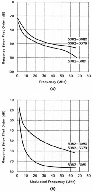
Figure 5-Typical second-order IMD (A) and cross-modulation distortion (B) responses of RF PIN diodes. Cross-modulation distortion, an effect also long untested in most Amateur Radio equipment reviews, is particularly important in these days of superpower shortwave broadcasters operating in and adjacent to Amateur Radio bands. Cross-modulation causes one signal's modulation to appear on other signals passing through the distorting device. (Conditions for A: 10-dB bridged-T attenuator; 40 dBmV output levels; one input frequency fixed at 100 MHz. Conditions for B: 10-dB bridged attenuator; 40 dBmV output levels; unmodulated frequency fixed at 100 MHz; variable frequency 100% modulated by 15-kHz audio.)
Notes
- This figure assumes that the IMD comes from equal-level input signals.
- This figure also assumes equal-level input signals.
- D. DeMaw and G. Collins, "Modern Receiver Mixers for High Dynamic Range," QST, Jan 1981, pp 19-23.
- This characterization of blocking differs from what we call blocking in ARRL Lab receiver testing for QST Product Reviews. We define a receiver's blocking dynamic range as the difference, in decibels, between the signal power that produces a 3-dB signal-plus-noise to noise ratio (in other words, the receiver's minimum discernible signal [MDS]) and the power of an out-of-passband signal that reduces the audio output produced by a desired signal (at a level 10 dB below the radio's 1-dB compression point for radios with their AGC turned off, or equal to 20 dB above MDS for radios with AGC that cannot be turned off) by 1 dB. This measurement indirectly reflects the purity of the oscillators involved if they are so noisy that reciprocal mixing raises the receiver noise floor enough to mask the onset of blocking. When this occurs, we characterize that measurement as noise limited and denote it as such in the Product Review. -Ed.]
- Purists considering "S units" in terms of the RST signal-reporting system (in which the lowest S number is 1) may insist that there is no such thing as "S0," but we have not exhausted the communication possibilities afforded by today's real-world radio links by the time we've worked downward to S1 on a 6-dB-per-S-unit basis from the decades-old amateur "standard" of S9 = 50 µV in 50 Ω. Solid communication can often be established and maintained at signal levels too weak to move our S meters.-Ed.]
References
- D. Mercy, "A Review of Automatic Gain Control Theory," Radio Electronics Engineering, Vol 51, p 579, Nov/Dec 1981.
- H. Nyquist, "Regeneration Theory." Bell System Technical Journal, Vol I I, p 126, Jan 1932.
- J. Ohlson, "Exact Dynamics of Automatic-Gain Control," IEEE Transactions, Vol COM22, p 72, Jan 1974.
- B. Oliver, "Automatic Volume Control as a Feedback Problem," IRE Proceedings, Vol 36, p 466, Apr 1948.
- W. Victor and M. Brockman, "The Application of Linear Servo Theory to the Design of AGC Loops," IRE Proceedings, Vol 48, p 234, Feb 1960.
- U. Rohde and T. Bucher, Communications Receivers, Principles and Designs (New York: McGraw-Hill Book Company, 1987).
KA2WEU, Dr Ulrich L. Rohde.