How to maximize your receiver's effective selectivity 1
Are you blaming other hams for interference that could be eliminated if you really knew how to operate your receiver? Is band noise irritating? Effective use of your receiver's selectivity features can reduce or eliminate much of the interference and noise that's been spoiling your fun.
To get the best performance from your receiver on the busy and often noisy MF and HF bands, you need to know a few things that your receiver's operating manual may not cover in detail. With the aid of several graphs, I hope to provide you with that information. For additional insight, I recommend you read two excellent, previously published QST articles that discuss receiver performance: one written by George Collins, KC1V, and the other by David Newkirk, WJ1Z(1)(2)
Some Fundamentals
The way a receiver's front-end stages operate significantly affects the IF-stage filters' ability to reject interfering noise and signals. The first step toward better reception is understanding that undesired signals and noise must be attenuated as much as possible before they reach the receiver's detector stage. These reductions should be accomplished without sacrificing desired-signal readabiIity. To do this intelligently, you need to understand your receiver's selectivity characteristics. You'll find that if the interfering signals are weak compared to the desired signal, you might even eliminate interference from signals that are on the same frequency as the desired signal!
Remember this simple fact: Filters work best if the signals applied to them are weak. Some receivers typically exhibit higher gain on the MF and lower HF bands than they do on the higher bands. Additionally, the atmospheric noise level on the MF and lower HF bands is generally high and might even be considered negligible on the upper HF bands. Because you can't hear signals that are below the noise level at the receiver's input, it simply makes no sense to allow your receiver's front-end stages to amplify anything below that level. Often, you can use your receiver's attenuation and RF gain controls to reduce the noise level reaching the IF filters to a level so low that the noise will not pass through the filters at all, while the signal you want goes straight through to the detector. Under these conditions, the receiver's filters also do a betterjob of removing adjacent frequency interference. I'll illustrate this process by using graphs that show the relationships between signal and noise amplitudes appearing at the IF-filter input and what the filters pass and reject.
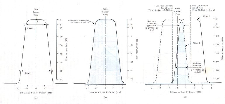
Figure l - At A, the response curve of a TS-940S SSB filter plotted from the manufacturer's selectivity specifications. At B, the overlaid response curves of two TS-940S cascaded filters. At C, the passband of filter 1 is shifted up 700 Hz from the filter center frequency; the passband of filter 2 is shifted down 1500 Hz to achieve the minimum effective bandwidth of the filter combination.
These graphs are based on the following specifications: recelver selectivity set for SSB with a passband 2.4 kHz wlde at -6 dB and 3.6 kHz at -60 dB. The aan SLOPE TUNE controle are set for a high cut of 1500 Hz or more end a low cut of 700 Hz or more.
Filter Specifications and Representative Response Curves
Let's analyze the IF-passband selectivity figures included in the specifications for the receiver section of a pair of transceivers. I'll discuss the variable bandwidth tuning (VBT) feature of the Kenwood TS-940S and the passband tuning (IF Shift) of the Kenwood TS-440S as used during SSB reception.
For the first example, VBT, I'll use the specifications given for-the Kenwood TS-940S HF transceiver.(3) The radio's SSB receiving selectivity listed as 2.4 kHz at -6 dB and 3.6 kHz at -60 dB .(4) These numbers define five points that can be plotted two different ways to illustrate the receiver's selectivity characteristics. Often, this information is plotted as a filter-response curve, as shown in Figure IA. Point A on the curve is not normally listed in selectivity statements, hut it's safe to assume that the zero-attenuation point of a filter lies at the center ot' its response curve. Points B and C define the width of the response curve at a level 6 dB below the 0-dB attenuation point. Points D and E define the filter response curve width at 60 dB below the 0-dB attenuation point on the curve. Lines drawn between points A through E approximate the filter response curve. The shape of the curve beyond the 60-dB attenuation points is not defined by the usual -6dB/-60dB selectivity statement and cannot be accurately plotted from that information. lt's realistic to assume, however, that the selectivity curve becomes fairly horizontal at each side of the bottom of the response curve, perhaps somewhere between -70 dB and -80 dB. Even so, a very strong adjacent signal might bypass the filter (a phenomenon known as "filter blow-by") if that 70 to 80-dB attenuation level isn't sufficient to eliminate it.
This filter-response curve can be used to analyze the combined bandwidth of two filters used in the TS-940S receiver IF stages. The first filteroperates, at in 8.83-MHz IF; the second filter operates at a 455-kHz IF. These two filters are cascaded, working together to form the equivalent of one filter with the characteristics similar to that of the hypothetical filters shown in Figure 1B. In the TS-940S, these cascaded filters produce a form of VBT referred to as SSB slope tuning. In SSB slope tuning, one filter passband can be shifted up in frequency and the other filter passband can be shifted down in frequency, effectively narrowing the bandwidth of the combined filters. This operation is illustrated in Figure IC.
As mentioned earlier, if we're trying to remove interfering signals at our receiver's IF stages, it makes sense to amplify the interfering signals and noise as little as possible before they reach the IF amplifiers. lt is also advantageous to attenuate interfering signals and noise as much as possible before they reach the receiver's RF amplifier. Signal strength and amplification are commonly plotted with zero signal strength at the graph bottom, with signal strength increasing vertically. In this presentation, I've inverted the filter-response curve so that the effects of attenuation, signal strength and amplification are plotted on the same graph, with the zero-attenuation point of each curve at the graph bottom. By inverting a filter-response curve, we produce a filter selectivity curve or an attenuation curve.
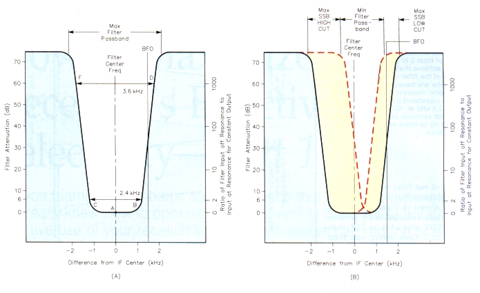
Figure2 - SSB selectivity curves for a Kenwood TS-940S transceiver with varlable bandwidth tuning.The curve at A is the result of setting the SSB SLOPE HIGH and LOW controls at minimum. At B, the resultant curve with the SLOPE HIGH end LOW CUT controle set at maximum: 1500 and 700 Hz, respectively.
I'll use the attenuation-curve format for the graphs shown here because it is easier and more obviously meaningful to plot signal shapes and signal magnitudes against filter characteristics. In Figure 2A, I've inverted Figure 1A to produce an attenuation curve. In this figure, the transceiver's SSB SLOPE TUNE controls (HIGH CUT and LOW CUT) are set at minirnum. The shaded areas emphasize what the filters reject.
Figure 2B shows both of the receiver's SSB SLOPE TUNE controls set at maxirnum. In this graph, you can see that these maximum SSB SLOPE TUNE control settings produce an extremely narrow passband that would be pretty good for CW, but is much too narrow for SSB because too much audio is eliminated from the desired signal. I've added the BFO frequency to Figure 2B to show the relationships between the SSB SLOPE TUNE HIGH CUT and LOW CUT settings and the BFO frequency.
When the TS-940S is in SSB mode, the BFO frequency is fixed. During SSB reception, the BFO signal replaces the suppressed carrier of the transmitted signal, being injected at the product detector after the IF filter. We want the IF filter to pass the desired sideband signal and reject everything else, including any small part of the suppressed carrier it might receive. The bandwidth of the IF filter is 2.4 kHz at the -6 dB points and the received sideband signal should be approximately centered within the IF-filter passband. Therefore, the BFO frequency must be offset 1.5 kHz (half the 2.4-kHz passband) from the IF-filter passband to produce the correct audio frequencies at the product detector. An SSB signal is considerably wider than a CW signal. There fore, when using the same IF filter in the CW mode, the BFO frequency is offset about 800 Hz from the IF-filter passband to produce an 800-Hz tone with the CW PITCH control set at its center position.
For the second example, IF Shift (passband tuning) SSB filters, I've used the specifications for the Kenwood TS-440S HF transceiver (see Figure 3A). Here, the receiver's SSB selectivity is listed as 2.2 kHz at -6 dB and 4.4 kHz at -60 dB. Using these numbers, I created a graph similar to that of Figure 2A. Note that this filter passband is narrower at the bottorn of the curve and wider at the top than that of the TS-940S. The TS-440S filtering system is different from the VBT scheme used in the TS-940S. With the TS-440S, you cannot change the passband shape, but you can shift the passband up or down in frequency as shown in Figures 3B and 3C. Shifting the passband up or down in frequency does not change the frequency relationship between the BFO and the desired signal, so the desired signal sounds normal.
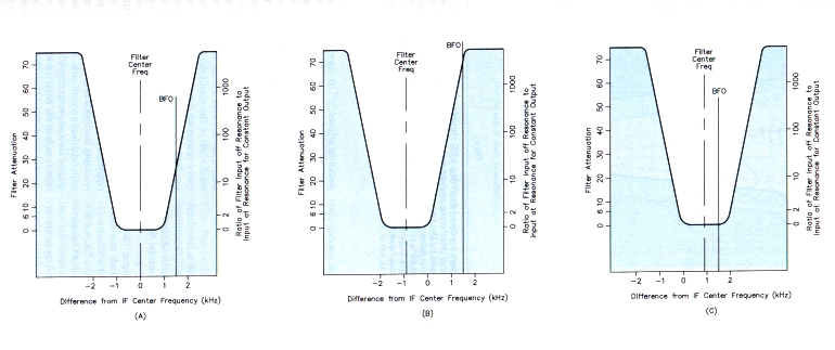
Figure 3 - SSB selectivity curves of a Kenwood TS-440S transceiver with passband tuning (IF SHIFT). At A, the selectivity curve with the IF Shift set at zero. Graph B shows the selectivity curve with the IF SHIFT set at -900 Hz. At C, the IF SHIFT is set at +900 Hz.
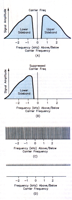
Figure 4 - At A, a double-sideband AM signal. An SSB signal Is shown at B. At C, a representation of noise at end around a given operating frequency. An abbrevlated graphical representation of broadband noise is shown at D.
Examining filter performance
Now we'll start adding representative signals and noise levels to the receiver filter curves to visualize how the IF filters perform under different circumstances. The voice information in an AM signal is contained in two sidebands, one above carrier and a mirror image below the carrier (Figure 4A). An SSB signal (as shown in Figure 4B) has but one sideband and the carrier is suppressed. These examples assume that the signal is modulated by a voice having more low frequencies than high. In these cases, most of the audio-derived energy of the signal is concentrated near the carrier. With a voice having greater high-frequency content, more audio energy is farther away from the carrier. Why is this important when considering receiver SSB selectivity? Because the optimum settings of the SSB SLOPE TUNE controls (for VBT) or the IF SHIFT control (for passband tuning will be somewhat different when listening to a high-pitched voice. In Figures 4A and 4B, the signal intensities are plotted vertically, so that stronger increments stretch higher on the graph than weaker increments do. The shape of an SSB signal with a high-pitched-voice might interact somewhat differently with the selectivity curves.
Being more concerned about effective communications quality audio than high fidelity allows us to make a signaificant reduction in audio bandwidth without sacrificing readability. We can use our receiver's selectivity controls to eliminatenate some of the unneeded audio highs and lows of the desired signal and thereby reduce or eliminate interference.
Noise
Much noise is broadband noise. The amount of noise your receiver responds to is proportional to the bandwidth used:
Halving your receiver's bandwidth should result in halving the received noise power and so on. Static field strength appears, on average, to be approximately inversely proportional to frequency. The higher the frequency, the less statie you have to contend with. On the MF and lower HF bands, noise is generally less severe during daylight hours than at nighttime because of varying band conditions, unless you have nearby thunderstorms.
Refer to Figure 4C, a graphical representation of noise at and around a given operating frequency. This graph can represent a broad bandwidth or mixture of individual random high, medium and low-intensity noise spikes. Because most of the lower- and medium-level spikes in this mix are overwheimed by the higher-intensity spikes, the former can largely be ignored, allowing use of an abbreviated graphical representation of broadband noise (Figure 4D) in Figures 5 through 7. I use this abbreviated representation to avoid cluttering the graphs below the applicable upper levels of noise.
Getting the Most from VBT Filters in IF Stages
Now that the groundwork is laid, let's examine how we can reduce or eliminate interference and noise under different representative situations we might encounter on the bands. Our first situation using a TS-940S (labeled Situation 1) involves two adjacent interfering signals and is illustrated in Figures 5 and 7. In Figure 5A, we assume that with TS-940's RF ATTenuator set to 0 dB and its RF gain control set at maximum, the noise level appears at +40 dB in the IF passband filters. (This is not an unreasonable assumption for nighttime reception en 75 meters.) We are trying to receive an LSB signal, which peaks at a level 25 dB above the noise. There are two equally strong LSB signals, one 2 kHz above and one 2 kHz below the desired signal.
In this graph, and in all the following graphs that relate to the use of VBT filters, the overall unadjusted bandwidth of the filters is shown. This clearly shows the effects of changing the settings of the SSB SLOPE TUNE controls. The righthand side of the unadjusted selectivity curve relates to the minimum setting of the SSB SLOPE LOW CUT control; the left-hand side of the unadjusted selectivity curve relates to the minimum setting of the SSB SLOPE HIGH CUT control. Where the LOW CUT and/or HIGH CUT controls are used to decrease the effective bandwidth of the filters, curves representing the upper and lower sides of the adjusted bandwidth are shown. The shaded area (representing what the filters reject) ends at the adjusted lower and upper sides of the effective-selectivity curve. This makes the effects of the LOW CUT and HIGH CUT control settings very obvious.
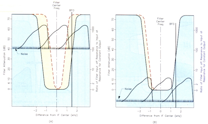
Figure 5 - Situation 1, using a TS-940S with SSB SLOPE TUNE control. There are two interfering LSB signals, one 2 kHz above and one 2 kHz below the desired signal. The signal strengths of the desired and interfering signals are equal, both peaking 25 dB above the noise. The recelved nolse In this and subsequent graphs is represented by the heavy horizontal line at the zero-signal levels of the other signals. At A, the recolver's input attenuator and RF gain controls have not yet been adjusted to eliminate the interfering signals. The LOW CUT ia Set at MAXIMUM (700 Hz); the HIGH CUT is set at 60% (900 Hz). Under these conditions, the interference from the signal down the band is eliminated, but within the passband there is some interference from the signal up the band and the noise level is high. At B, the recelver's attenuator and RF gain controls have been adjusted to maximize rejection of the interfering signals and nolse. The LOW CUT is set at zero; the HIGH CUT is set at 21% (314 Hz).
As you can see in Figure 5A, with the ATTenuator control set to 0 d8, the RF gain control at maximum and the SSB SLOPE HIGH CUT and LOW CUT controls set at minimum, we have severe interference from both adjacent-frequency signals and the noise is objectionable.
Before we use the two SSB SLOPE TUNE controls, let's examine their operation. The LOW CUT and HIGH CUT controls are used to narrow the filter passband by moving the sides of the selectivity curve toward the filter center frequency. How do you know which control to use and what to expect? It's simple: If the interference is low-pitched, use the LOW CUT control to move the side of the curve nearest the BFO frequency closer to the passband center frequency (and away from the carrier frequency) by as much as 700 Hz. This reduces or elirninates the low-pitched interference and also cuts some of the lows from the audio of the desired signal. If the interference you hear is high-pitched, use the HIGH CUT control to move the side of the curve farthest from BFO frequency closer to the passband center frequency (and eloser to the carrier frequency) by as much as 1500 Hz.
Figure 5A shows that we can use the HIGH CUT and LOW CUT controls to eliminate interference from the signal 2 kHz lower in frequency, but we can't eliminate all the interference from. the signal higher in frequency. In Figure S5, the noise is at about the 40-dB level on the selectivity curve. The filter bandwidth at the 40-dB point of the curve is about 3.16 kHz wide with the HIGH CUT and LOW CUT controls set to zero. With the HIGH CUT and LOW CUT controls adjusted as shown in figure 5A, the resulting bandwidth at the 40-dB level on the curve is about 1.52 kHz. Therefore, the HIGH CUT and LOW CUT controls have reduced the effective bandwidth to about 48% of the original. Because the noise is broad-spectrum noise, this bandwidth reduction should result in cutting about 3 dB of the noise that passes through the filters. If the signal you're trying to copy is down in the noise, this action may make the signal somewhat more readable.
Now look at Figure 5B. You can slide the signals and noise down the selectivity trough by adjusting the ATTenuator control to maximum (30 dB) and reducing the RF gain. You can now set the LOW CUT and HIGH CUT controls as shown in this graph. This eliminates the noise and the interferencefrom both interfering signals. Yes, we have reduced the received-audio bandwidth of the desired signal to about 1700 Hz, hut now you can copy with no interference and the received audio is still of acceptable communications quality. Any noise you might now hear is caused by noise generated within the receiver and is much less objectionable than the static crashes and other racket that is arriving at the receiver's antennajack. In many cases, all you now hear is the signal you want to hear. Yes, you may have to turn up the audio gain and the S meter doesn't work, but so what? You got rid of the interference! With these things in mind, isn't it kind of dumb to let the receiver run wide open with no signal attenuation and the RF gain control set at maximum?
The second situation using a TS-940S (labeled Situation 2 in the graphs) involves two extremely strong adjacent interfering signals; this is illustrated in Figures 6A and 6B.
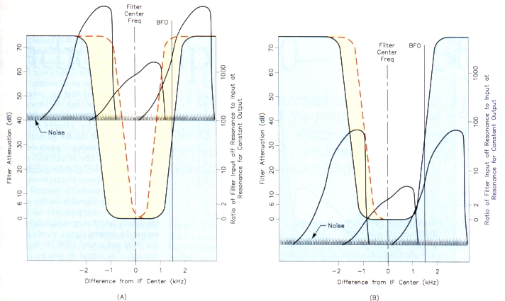
Figure 6 - SItuation 2, using a TS-940S with SSB SLOPE TUNE control. Both graphs show two lnterfering eignals, one 2 kHz above end one 2 kHz below the desired signal. The desired signal peaks 25 dB above the nolse (represented by the heavy horizontal bar). Both interfering signals are 25 dB stronger than the desired signal. At A, the input attenuator end RF gain controls are wlde open.
The LOW CUT is set at maximum (700 Hz) and the HIGH CUT is eet at 71% (1072 Hz). In this case, peaks of the high-intensity interfering signals pass right by ("blow by") the IF filters. The lower-level portions of the up-band signal are within the passband end the noise level is high. At B, by proper adjustment of the input attenuator and RF gain controle, the interfering signals end the noise have been eliminated-pushed right out of the passband. Here, the LOW CUT Is set at zero; the HIGH CUT Is set at 42% (623 Hz).
Let's examine what happens when the signal we want is sandwiched between LSB signals, both 25 dB stronger than our desired signal, one 2 kHz up the band and one 2 kHz down the band. See Figure 6A. Here we again assume that the receiver's ATTenuation control is set to 0 dB, the RF gain control is set at high and the noise level appears at the 40-dB level of the filters. The situation is similar to that we saw in Figure 5A, only much worse. Even setting the LOW CUT control at maximum will not eliminate part of the interfering signal up the band that falls near our BFO frequency. Setting the HIGH CUT control as shown in this graph eliminates an insignificant portion of the interference from the signal down the band. However, the interference that might be eliminated by narrowing the passband of the filters is insignificant compared to those parts of both interfering signals that are so strong that they blow right by the IF filters and reach the product detector. We still have very strong interference from both interfering signals as well as objectionable noise.
Refer to Figure 6B. Here, the receiver's ATTenuator is set at maximum (30 dB) and the RF gain control setting is reduced. This slides the three signals and the noise level down the selectivity curve to a point at which the noise and both interfering signals can be eliminated completely. The LOW CUT control can be set at zero and still elirninate the signal up the band, but it's necessary to use the HIGH CUT control to eliminate signal down the band. Compare this graph with Figure 5B. You will see that interference- and noise-free reception of a desired signal in the presence of two very strong interfering signals can be comparable to receiving the same signal in the presence of two interfering signals having the same strength as the desired signal.
The third situation using a TS-940S (Situation 3) involves interfering signals on or very close to the desired signal, but somewhat weaker than the desired signal. This is illustrated in Figure 7.
Referring to Figures 5B and 6B, you'll sec that in both cases we have eliminated the noise by using the ATTenuator and the RF gain controls to slide the noise below the flat bottorn of the selectivity curve. As shown in Figure 7, the same approach can often be used to eliminate interference frorn signals that are weaker than the desired signal and on, or very near, the same frequency as the desired signal. This is done by simply using the ATTenuator and the RF gain control to move the interfering signals below the flat bottom of the selectivity curve as shown in Figure 7. Of course, the audio of the on-frequency interfering signal would sound perfectly normal because the interfering signal is on the same frequency. Al] corriponents of the off-frequency interfering signal, being 1 kHz below the desired signal, would beat with the BFO and sound 1000 Hz higher than normal; this signal would be unintelligible and annoying.
Part 2 of this series will discuss passband tuning as used in the Kenwood TS-440S.
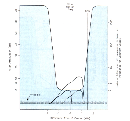
Figure 7-Situation 3, using a TS-940S with SSB SLOPE TUNE control. The desired signal peaks 25 dB above the noise level. There are two interfering signals, one on the same f requency as the desired signal, the other 1 kHz below the desired signal. Both interfering signals are 12.5 dB above the noise. Aqain, the Input ATTenuator end RF gain controle have been adjusted to elimlnate the Intertering signals end the noise. The LOW and HIGH CUT controle are set to zero.
Notes
- George Colijns, KC1V, "Receiver Features that Help You Beat lnterference", QST, Feb 1983, pp 43-47.
- David Newkirk, M 1 Z, "Transceiver Features that Help You Beat lnterference". QST, Mar 1991, pp 16-21.
- Bruce 0. Williams, WA61VC, "Trio-Kenwood Communications TS-940S HF Transceiver", Product Review, QST, Feb 1986, pp 47-49.
- The numerical result obtained by dividing the -60 dB bandwidth by the -6 dB bandwidth is known as the filter's shape factor, the smaller the number, the better the shape factor. In this case, the TS-940S filter's shape factor is 1.5
W4QEJ