Simplified design of inductively-coupled circuits
Calculations for resonant and nonresonant secondaries.
If you are having trouble loading your I inal with link coupling or in driving an amplifier using inductive coupling, a few calculations using simple algebra and a deck with a g.d.o. can give you the reason and tell you what can be done about it.
One important class of coupling networks often used by the amateur experimenter was not treated in George Grammer's client three-part article(1) on impedance-matching networks. This class includes the magneticupled interstage or output circuit still found in any transmitters. This is especially true of the tput circuit of balanced push-pull amplifiers. oo often the design of these networks proceeds a cut-and-try fashion; the designer selects a stable inductance which resonates with the output and tuning capacitance of the tube. Then he experiments with several links until he can couple rated power from the tube. The step-by-step design procedures outlined below will obviate most of the experimenting in a majority of cases. Three types of magnetic coupling circuits will be considered: (1) the parallel-resonant primary with series-resonant secondary, (2) the parallel-resonant primary with parallel-resonant secondary, and (3) the parallel-resonant primary with untuned secondary. These three cases cover most of the amateur applications. Magnetic coupling and the measurement of coupling coefficient with instruments readily available to the average amateur will also be discussed.
Parallel-resonant primary and series-resonant secondary
The first circuit to be considered is shown in Fig. 1. This is a typical link-coupled output stage. The primary circuit consists of the usual parallel LC resonator, while the secondary circuit is the series-tuned resonator often found in link output circuits. Both the load resistance, R2, and the output resistance of the tube, R1, are generally known. The load resistance is usually low (between 50 and 100 ohm). The output resistance of the tube is usually high (between 1000 and 10,000 ohm). The output resistance can be roughly approximated by the formula
![]()
where:
En is the rated anode supply voltage
Emin is the minimum anode voltage during the r.f. cycle
Po is the rated power output of the tube.
The objective is to design a magnetic coupling network which will permit the tube to deliver maximum power to the load, R2, at a chosen frequency. At the same time, it is necessary to be certain that the circuit will discriminate against harmonic and subharmonic frequencies and not require too large a value of coupling coefficient between the primary and secondary coils, L1 and L2.
The circuit will discriminate against unwanted frequencies if a large enough operating Q for the primary circuit is chosen. The operating Q is defined as the Q of the primary circuit alone. This may be as low as 5 or as high as 20, but values between 10 and 15 are usually the best. If the value chosen is too high, the tank-circuit efficiency will be reduced. However, at the higher frequencies the minimum operating Q may be limited by the irreducible output capacitance of the tube.
The maximum coupling coefficient between practical air-core solenoids is usually 0.4 or less. Measurements made by the author on the B & W JEL 40, 20, and 10 fixed-link tank coils exhibited coupling coefficients between 0.35 and 0.415. A Bud 40 meter swinging-link tank coil had a coupling coefficient of 0.3 with the link close to the primary coil. A simple method of measuring the coupling coefficient with a grid-dip meter or a Q meter is given later on.
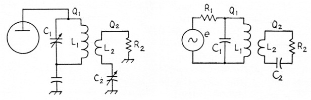
Fig. 1. Low-impedance (link) output circuit with resonant secondary.
Given R1 and R2, the step-by-step design procedure for the circuit in Fig. 1 is:
1) Select the primary-circuit operating Q, Q1. (Usually between 10 and 15.)
2) Calculate ![]()
3) Calculate ![]()
(For Q1 greater than 5, XL1 and XC1 differ by less than 4 per cent.)
4) Select the coupling coefficient ![]()
(This should be less than 0.4. For swinging links, choose k less than 0.3.)
5) Calculate the secondary Q, ![]()
6) Calculate ![]()
7) Calculate C1, L1, C2, and L2 from the values of XC1, XL1, XC2 and XL2 and the chosen frequency.
The proper spacing between primary and secondary coils can be determined experimentally when making the coupling-coefficient measurement. (See latter part of article for this measurement.)
This type of coupling circuit is best suited for output coupling where the ratio R1/R2 is a large number. For interstage-coupling networks, where the impedance ratio is small, the circuit of the next section is often more suitable.
Parallel-resonant primary and parallel-resonant secondary
The remarks concerning the operating Q and the largest realizable coupling coefficient made in the preceding section also apply here. This circuit is well suited for interstage coupling because the shunt capacitance of the grid can be absorbed in C2. Fig. 2 shows the circuit diagram and the equivalent circuit.
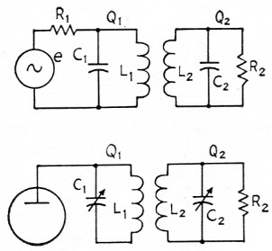
Fig. 2. Circuit for coupling inductively to a high-impedance load.
Given R1 and R2, the design procedure in this case is as follows
1) Select Q1.
2) Calculate ![]()
3) Calculate ![]()
4) Select k (less than 0.4).
5) Calculate ![]()
6) Calculate ![]()
7) Calculate ![]()
8) Determine C1, L1, C2, L2 and experimentally determine the coil spacing by making the coupling-coefficient measurement.
An alternate procedure is to select Q1 and Q2 and then calculate the required value of coupling coefficient. If it is not too large, proceed with the design.
Parallel-resonant primary and untuned secondary
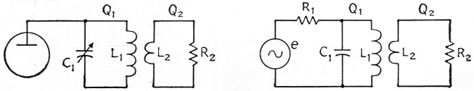
Fig. 3. Low-impedance (link) coupling with non-resonant secondary.
This circuit is shown in Fig. 3 and may be used when resonating the secondary is not desired. The design steps are:
Given R1 and R2,
1) Select Q1 and set Q2 = 1.2.
2) Calculate ![]()
3) Calculate ![]()
4) Calculate ![]()
5) Calculate ![]()
If k is greater than 0.4 select higher values of Q1 until k is less than 0.4. It can be shown that, for 5 < Ql < 20, k will be minimum when Q2 is approximately 1.2.
Experimental determination of coupling coefficient
The coupling coefficient between two coils scan be determined easily using only a grid-dip oscillator or a Q meter. The chief advantage of the method to be described is that the measurement can be made at or near the actual operating frequency of the coils. The grid-dip meter and Q-meter measuring circuits are shown in Figs. 4A and 4B, respectively.
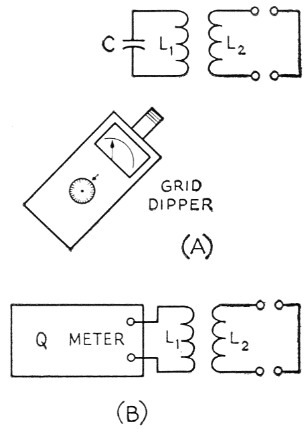
Fig. 4. Methods of determining the coefficient of coupling, using a grid-dip oscillator (A) and Q meter (B).
The measurement procedure using "the grid-dip meter is as follows:
1) With L2 open-circuited, resonate L1 with C at the desired frequency, 10. Make sure that leads are kept as short as possible.
2) Short-circuit L2 by soldering its ends together and, with the same C, measure the new resonant frequency f.
3) Calculate ![]()
Note that fg will always be greater than fo because the effective inductance resonating with C when L2 is shorted will always be less than L1 alone.
The coupling coefficient can be adjusted to a desired value by the following procedure: After finding f calculate
![]()
and space L1 and L2 so that the circuit is resonant at f, when L2 is short-circuited. Grid-dip meter frequencies should, of course, be checked against an accurate standard.
The procedure with the Q meter is similar except that the resonant frequency is kept constant. The steps are:
1) Resonate L1 at the desired frequency with L2 open-circuited. The value of the resonating capacitance is Co and is read from the Q-meter capacitance dial.
2) Short-circuit L2 and re-resonate the circuit with the capacitance Cs, also read from the capacitance dial.
3) Calculate ![]()
Cs will always be greater than Co for the same reason as given before.
If k and Co are known, the required Cs can be found from the equation
![]()
The values of L1 and L2 can be determined experimentally with known capacitors at or near the design frequency. Always make sure that neither coil is short-circuited when this measurement is made.
Conclusions
The author has used these design techniques at frequencies up to 100 Mc with remarkable success. Once the amateur designer gets a "feel" for designing for a specified coupling coefficient and knows the upper limit of this parameter, exact design is fairly easy to accomplish. Most of the author's experience has been with the B & W Miniductors. Coils are cut from the coil stock which have the required inductance. Then the spacing between coils is experimentally determined by the grid-dip meter or Q-meter measurement. When the proper number of turns per coil and the spacing are known, a new transformer can be made by removing turns from the middle of another Miniductor without breaking the polystyrene, so as to give the required coil spacing. Then the ends of the Miniductor are cut off to give the proper number of turns for L1 and L2. This results in a mechanically rigid transformer which will not get out of shape under vibration or shock.
Notes
T.J. Maresca, W2VLA.